Have you ever felt you are losing too much time in traffic? Have you ever asked why all the cars on the roads can’t just all go with some constant speed? Most drivers have had such thoughts. And if you live in a large city, you may relate to this funny scene from “Office Space”:

In this post, we will present a mathematical model of traffic congestion and explain why it happens using this model. Afterwards, we will analyze the effects of a recently emerging and popular technology, autonomous cars, on traffic congestion. As we showed in our WAFR 2018 paper, “Altruistic Autonomy: Beating Congestion on Shared Roads”, autonomous cars have the potential of significantly reducing traffic congestion!

Background

Mathematical Model of Traffic

Decades ago, researchers came up with a beautiful model of traffic, and they called it Fundamental Diagram of Traffic (FDT). While it has several similar forms, the triangular model is widely adopted since it allows analytical investigation. The triangular model plots flow (the number of cars per second going through a point on the road) versus density (the number of cars per meter over some stretch of the road at any given second):

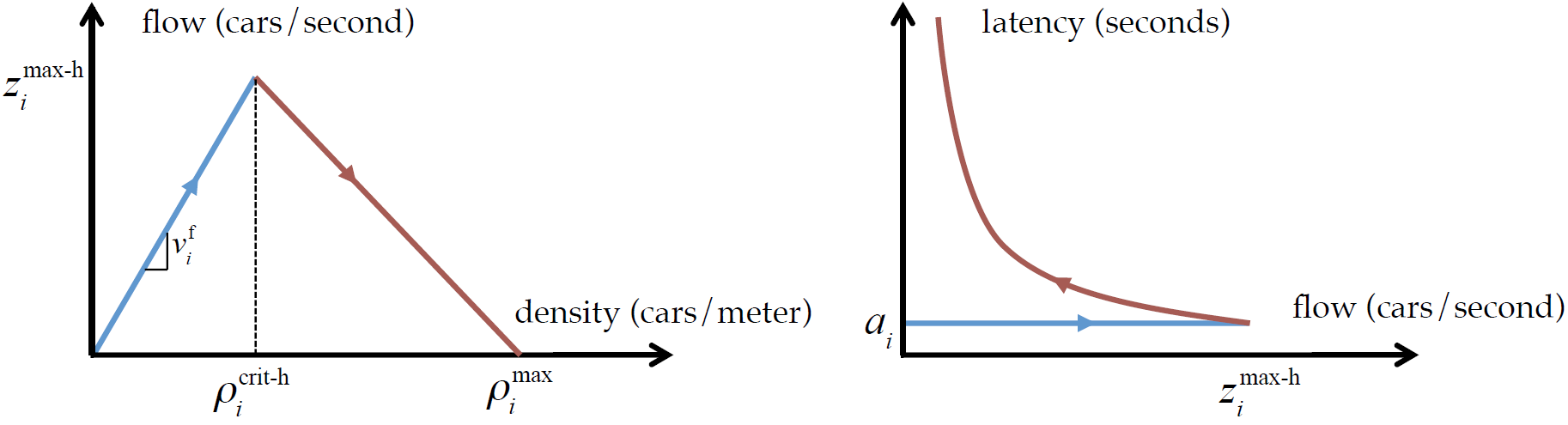
Fundamental Diagram of Traffic

Note the rising edge on the left (blue) and the falling edge on the right (brown). The rising edge represents the state of free-flow, where all cars can go with the maximum legally allowed speed. Imagine there is only a single car on the highway -- it would just go with the maximum speed. But, both traffic density and flow would be low, because after all it is just one car!

If we add a second car, they will still go with the maximum speed. Both density and flow will be doubled. However, we cannot just keep inserting new cars and expect them to go with the maximum speed. There is a rule: all drivers have to keep a distance of 2 seconds with the car in the front (so that they can respond in time in case the car in front unexpectedly brakes). Hence, at some point while inserting cars to the road, drivers will have to slow down or otherwise cars cannot fit to road. This is where we transition from the rising edge of the triangle to the falling edge, which represents the congested region. While the car density keeps increasing, the flow will now decrease because all cars are slowing down. This is shown by the second important plot of model, that of latency (the time it takes to travel from one point to another on the road) vs flow:

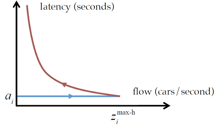
In the free-flow regime, latency is constant, since all cars are going with the maximum speed. However, as we increase density and move to the congested region, it rapidly increases.

Routing Problem

In its simplest form, the routing problem asks the following question: How do we allocate a given traffic flow (into N parallel roads) such that the total latency is minimized?

It may be confusing that we are given a traffic flow, not a traffic density. Although this might sound unintuitive, it becomes more and more sensible when you think about it: Would you enforce a constraint that states “there will be 500 cars on this road”, or a constraint “there will be 500 cars who want to go from point A to point B between 5pm and 6pm”? The latter one is more natural, and so used in the routing problem. We also simplify the traffic network as N parallel roads, which enables more mathematical analysis by ensuring we can use single density, flow and latency values for one road without any partitioning.

Nash Equilibria

Now, we can state the main cause of traffic congestion (and perhaps many other problems in the world): Humans are selfish. Imagine you live in Los Angeles, and want to go from Beverly Hills to the Valley. The shortest path you could take is Coldwater, which would normally take 25 minutes. The second best alternative is to take the highway 405, which would take 30 minutes. But it is Friday afternoon, so both Coldwater and 405 are congested and will take, say, 32 minutes. The other best alternative is to take Laurel, which is free of congestion. However, that road is long and the maximum speed is low, so it would already take 35 minutes.

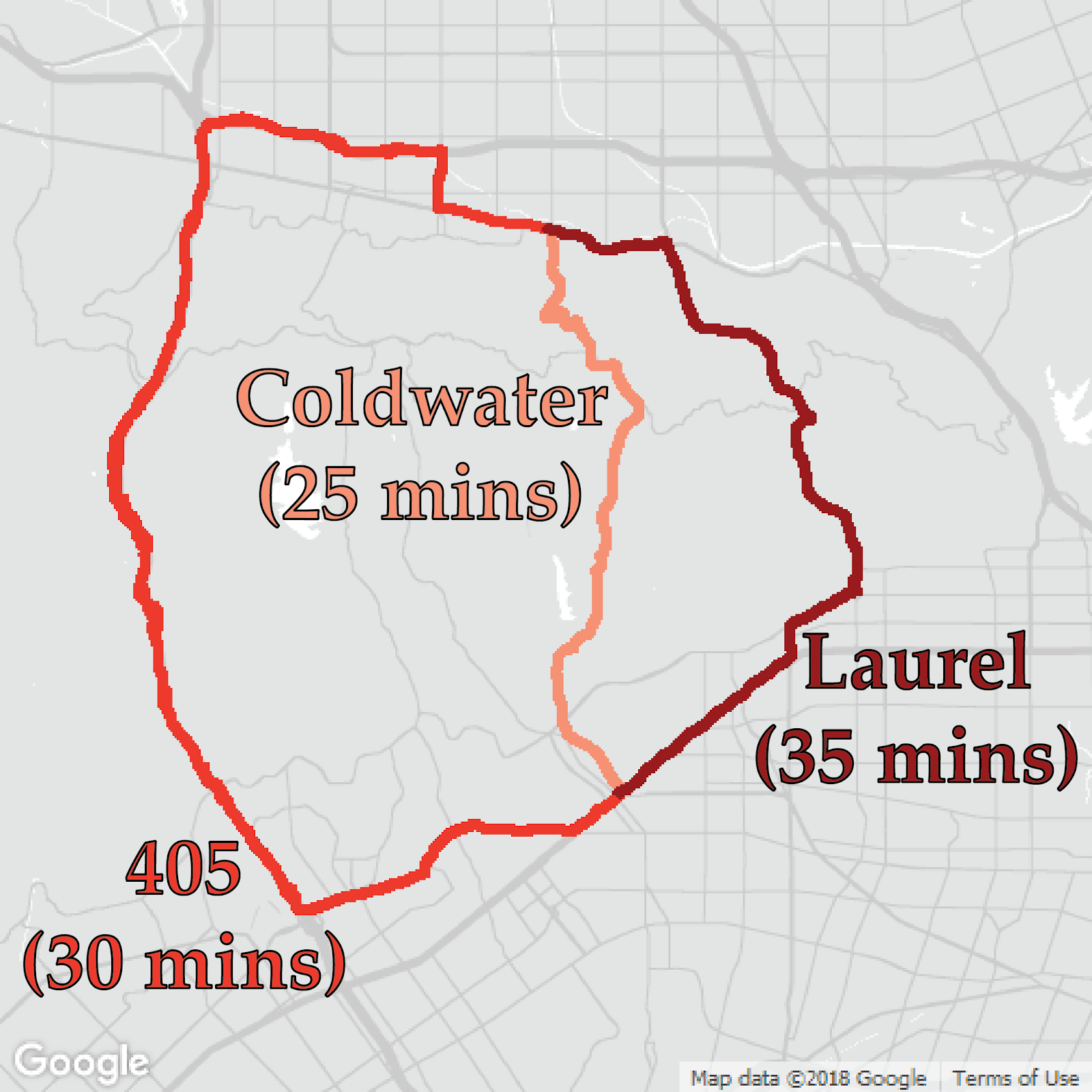
Then, you make your decision: You take Coldwater, because it is 3 minutes faster. But, you are not alone -- everybody does the same thing. Now sit back and think for a while: When you decide taking Coldwater, it was already congested. In other words, there were lots of cars taking that road. After you and many others decide to take it because it is 3 minutes faster for you, the road became even more congested - and will now take 34 minutes. It is still better than Laurel, isn’t it? If you (and others who made the same decision as you) had taken Laurel, you would have lost a few minutes, but hundreds of cars on Coldwater would have enjoyed a few minutes less travel time. You, along with many others, basically caused social bad, for your own good.

Well, we don’t blame you. This is Nash equilibrium (NE), where no car is willing to change the road it took, and you did what you are expected to do! As long as a road is faster than the others, people will choose to take it. So what’s the problem? The problem is Nash equilibrium is not unique and some of those equilibria can be really bad.

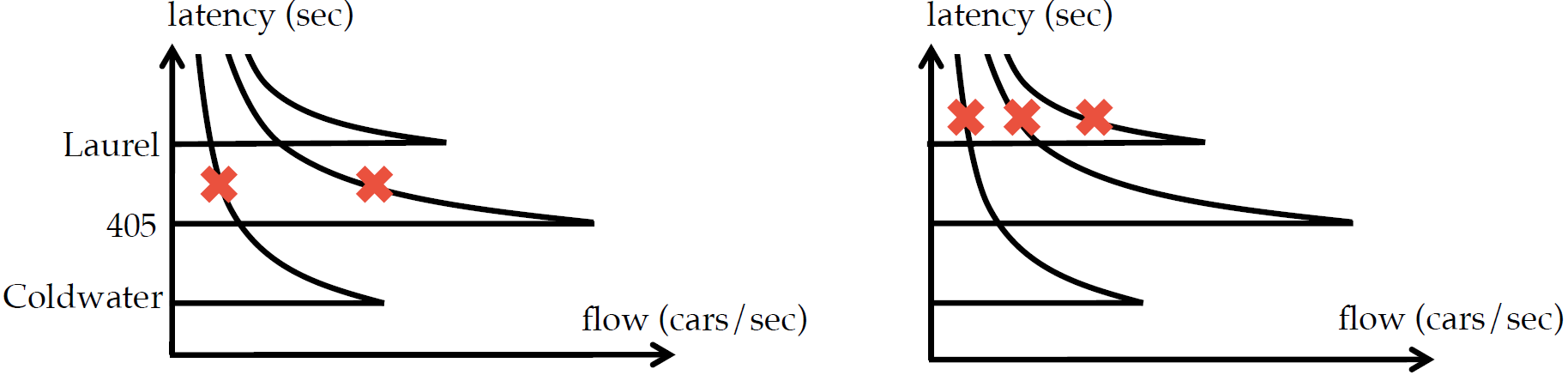
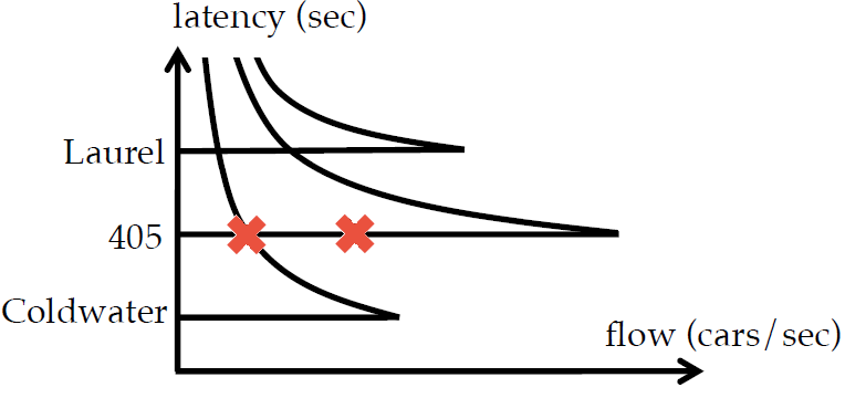
Two different Nash equilibria as solutions to the same routing problem.

If you look at these two flow-latency plots (note that each plot has the model of all three roads), you will see two different configurations. The crosses represent the state of the road. Both configurations are a Nash equilibrium, because all used roads have the same latency level, i.e. no drivers would benefit from changing the road they are taking. The surprising point is that they are both a solution to the [same]{.underline} routing problem -- the total flow in both configurations are exactly the same! However, in the second configuration drivers experience a much higher latency. With more complex and crowded networks, things can be unboundedly worse.

Best Nash Equilibrium

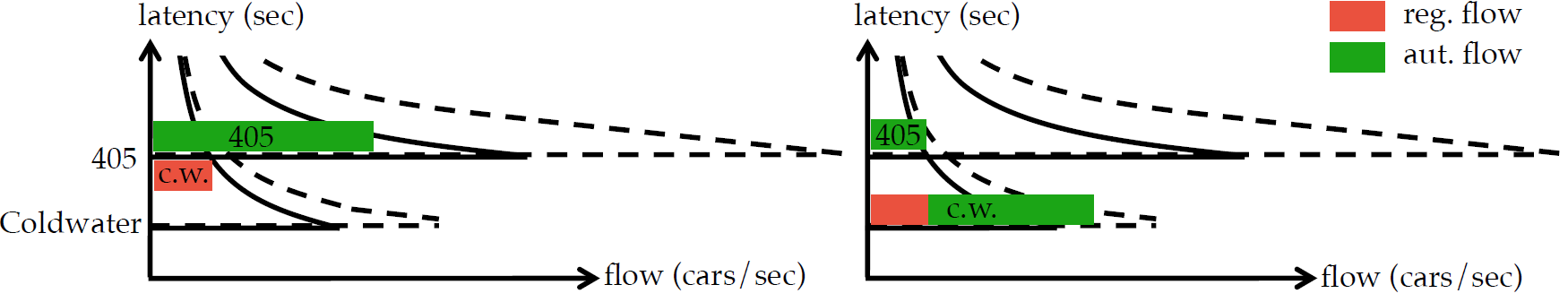
Among the Nash equilibria, which one or ones are the best? And what’s the criteria for being better than the others? You guessed it! The best Nash equilibria (BNE) are the ones that minimize the latency experienced by all drivers. So for example, in the previous figure, the first NE is better than the second one. Could it be better? Yes! In fact, we showed that in the BNE, one road has to be in free-flow¹, because otherwise we could just decrease the latency to the next highest free-flow latency road’s free-flow latency, and then easily adjust the flow values to match with the demand.

Best Nash Equilibrium for the above routing problem. 405 is now in free-flow.

So, what’s special about autonomous cars?

We said drivers have to keep a distance of 2 seconds, and it is because we need 2 seconds for our reflexes to, for example, brake. Autonomous cars do not suffer from this limitation. Of course, they still need some time, but it is around 1 second for autonomous cars, maybe even less.

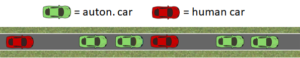
Autonomous cars can platoon, so more cars can fit on a road!

This brings about an interesting question: What happens to the FDT when all cars on the road are autonomous? What if we have a fixed ratio of autonomous and human-driven cars (we will call this ratio autonomy level)? We analyzed this and came up with the following modification:

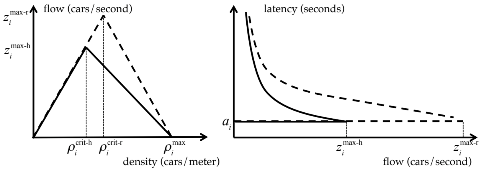
Two different FDTs are shown. Solid and dashed lines represent no autonomy and full autonomy, respectively.

So what happens is the critical density, the highest density where all cars can move with the maximum speed, increases. This also increases the maximum flow. However, the maximum density (a.k.a. jam density) does not change, because that point represents bumper-to-bumper traffic and it just depends on the lengths of the cars, not the headway. By increasing autonomy level, we basically move from the old FDT to the new one.

Robustness

The presence of autonomous cars has another important effect on the mathematical model of traffic. Since we can alter the autonomy levels of each road, we can have several BNE. So, which is the best among many BNEs? This sounds a little weird, because we know that all BNEs have the same latency level. So, we introduce a secondary metric: robustness.

In the routing problem, we assume we are given a flow demand. However, in real world, how possible is it to know the demand precisely? A small amount of unpredicted demand can be catastrophic and can lead to significant (in fact, unbounded) latency increase. Hence, we define the robustness as follows: A configuration is more robust than the other if it can allocate more extra flow demand with the same autonomy level, without increasing the latency. And this maximum extra flow demand is the quantization of the robustness. For example, in the BNE example above, the robustness value is the unused flow capacity of 405.

Then we define Robust Best Nash Equilibrium (RBNE) as the BNE that maximizes robustness. RBNE, too, is not necessarily unique.

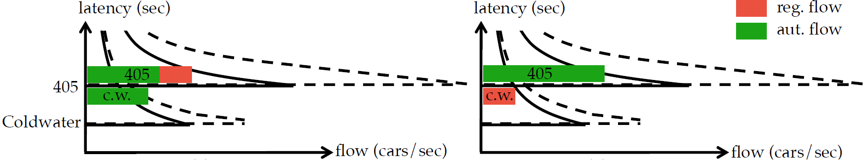
Two different BNEs with different robustness values.

For example, in the configuration above, the BNE at right is more robust, In fact, it is an RBNE. Because the 405 benefits more from autonomy than the Coldwater. Hence, a social planner can make the routing more robust to unforeseen demand by routing all autonomous traffic onto the 405.

Altruistic Autonomy

We said selfishness of humans is an essential cause of traffic congestion. The introduction of autonomy opens a new possibility: Can we have altruistic autonomous cars? Altruism can be obtained in several ways. For example, public transportation services can be altruistic -- buses can choose to take the longer route for the social good. Or ride-sharing services, e.g. Lyft or Uber, can offer lower prices to the customers in the cost of taking the longer route. When autonomous cars will be available for such services, these options could be further elaborated.

With this motivation, we define a mathematical altruism profile, which basically defines what portion of the autonomous cars accept what factor of altruism. For example, if 10% of the autonomous cars accept an altruism level of 1.5; this means one in every 10 autonomous vehicles accepts reaching its destination 1.5 times slower than the other -selfish- vehicles. This can greatly increase social utility. We define Best Altruistic Nash Equilibrium (BANE) to be the lowest total latency routing, given the altruism profile.

BNE is compared to the BANE with some modest altruism profile.

As you can see from the above figure, when a modest portion of the autonomous cars are altruistic, it is possible for majority of the cars to use the shortest route without causing congestion. This can significantly (in fact, unboundedly) decrease the total latency.

Mathematical and Algorithmic Contributions

Other than modeling the FDT with autonomy and analyzing several different NE, we presented algorithms in the paper that enables finding BNE, RBNE and BANE (with any altruism profile and autonomy level) in polynomial time. Our formulations are based on convex optimization, and can be very efficiently solved. For brevity, we do not give the full details in this blog post and refer to the paper.

Simulations and Results

We used SUMO traffic simulation package to simulate the roads with different autonomy level and altruism profile. We first evaluated our FDT model accuracy.

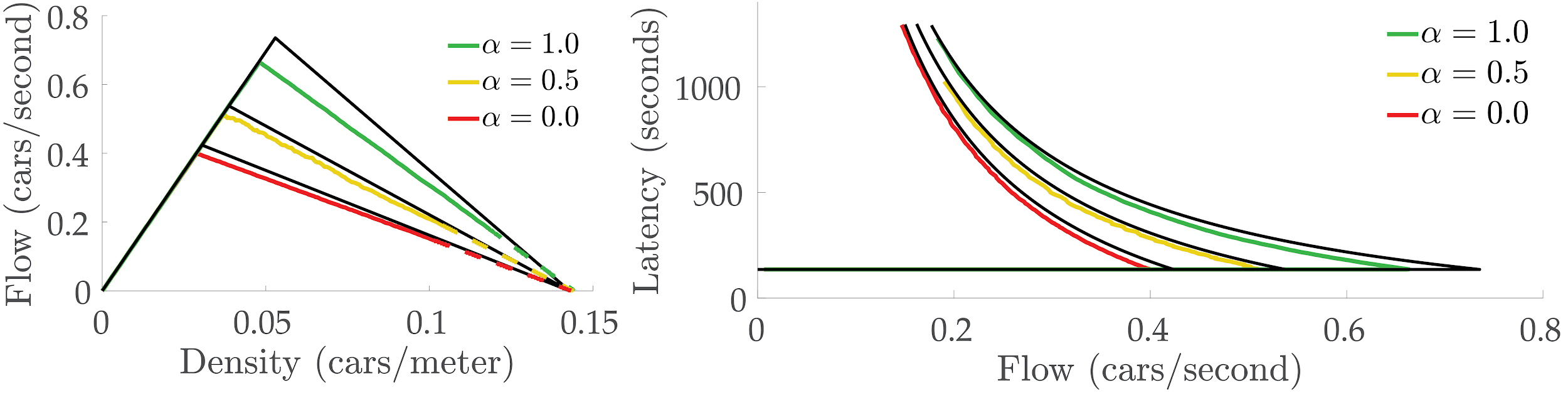
Theoretical FDT is compared to the simulation results. ⍺ represents the autonomy.

In the figure above, the black lines represent the theoretical values. While the simulation results and the theoretical values generally match, there is a small difference with increasing autonomy, which is because of the system imperfections in the simulator, such as the road shape and discretization.

In another experiment, we assessed how much gain we could expect from RBNE and BANE. We have seen that RBNE halves the total latency compared to a NE, and BANE can half it again! This means, with BANE, people can reach their destination in around 2 minutes, whereas they experience a latency above 8 minutes with the given NE. In fact, we showed that the improvement of BNE (or RBNE) over NE, and BANE over BNE can be unboundedly large!

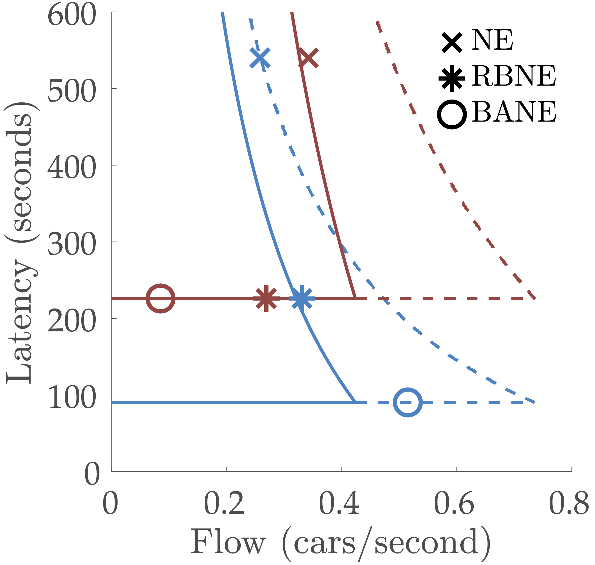
RBNE and BANE have the great potential to reduce latency on the roads.

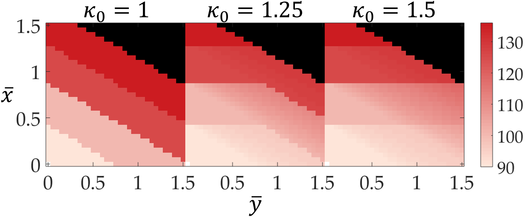
We also explored the effect of altruism level on a simple scenario where all autonomous cars have the same altruism level. In the heat-map below, colors represent the overall latency (black shows infeasibility), $\bar{x}$ and $\bar{y}$ denote the total regular and autonomous flow demand, respectively. And $\kappa_{0}$ is the common altruism factor. This first map has completely discrete latencies, as it has no altruism. With increasing altruism, the overall latency decreases and the insertion of extra cars does not hurt much.

Lastly, we have prepared a video that shows the improvements led by our equilibrium definitions. In this scenario, there are 4 roads between two points. Each road is shown as a single lane and we present the latency values in the video below.

Future Directions

In this post, we defined several important notions for traffic networks under mixed autonomy. We also presented algorithms for computing several different equilibria in the paper. For practical purposes, the following questions warrant further research:

• How can we use autonomy to move between equilibria?

• How can we build incentives for altruism?

• How can we use autonomy to deal with traffic disturbances such as accidents, closed lanes/bottlenecks, etc.?

• How does the results of this work extend to more general network topologies?

Hopefully, we can manage to tackle these further questions, and we shall all suffer slightly less from the stress caused by congested traffic.

References

Altruistic Autonomy: Beating Congestion on Shared Roads. E. Bıyık*, D.A. Lazar*, R. Pedarsani, D. Sadigh. 13th International Workshop on Algorithmic Foundations of Robotics (WAFR), December 2018

1. We assume no two roads are identical, otherwise the number of free-flow roads could be more than one. Also note that this statement is not bidirectional, i.e. having one road in free-flow does not guarantee that it is a BNE. ↩