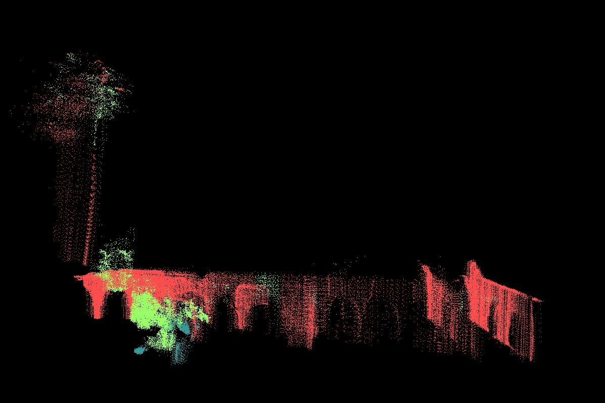
Terrain Classification

• Section from the paper describing the data and models
• Fly-thru movie of the AMN results
• Enlarged versions of test images in the paper
• Images of labeled potion of the test set

Our task is to classify the laser range points into four classes: ground, building, tree, and shrubbery. Since classifying ground points is trivial given their absolute z-coordinate, we classify them deterministically by thresholding the z coordinate at a value close to 0. After we do that, we are left with approximately 20 million non-ground points. Each point is represented simply as a location in an absolute 3D coordinate system. The features we use require pre-processing to infer properties of the local neighborhood of a point, such as how planar the neighborhood is, or how much of the neighbors are close to the ground. The features we use are invariant to rotation in the x-y plane, as well as the density of the range scan, since scans tend to be sparser in regions farther from the robot.

Our first type of feature is based on the principal plane around it. For each point we sample 100 points in a cube of radius 0.5 meters. We run PCA on these points to get the plane of maximum variance (spanned by the first two principal components). We then partition the cube into 3x3x3 bins around the point, oriented with respect to the principal plane, and compute the percentage of points lying in the various sub-cubes. We use a number of features derived from the cube such as the percentage of points in the central column, the outside corners, the central plane, etc. These features capture the local distribution well and are especially useful in finding planes. Our second type of feature is based on a column around each point. We take a cylinder of radius 0.25 meters, which extends vertically to include all the points in a "column". We then compute what percentage of the points lie in various segments of this vertical column (e.g., between 2m and 2.5m). Finally, we also use an indicator feature of whether or not a point lies within 2m of the ground. This feature is especially useful in classifying shrubbery.

For training we select roughly 30 thousand points that represent the classes well: a segment of a wall, a tree, some bushes. We considered three different models: SVM, Voted-SVM and AMNs. All methods use the same set of features, augmented with a quadratic kernel.

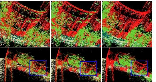
The first model is a multi-class SVM with a quadratic kernel over the above features. This model (right panel) achieves reasonable performance in many places, but fails to enforce local consistency of the classification predictions. For example arches on buildings and other less planar regions are consistently confused for trees, even though they are surrounded entirely by buildings.

We improved upon the SVM by smoothing its predictions using voting. For each point we took its local neighborhood (we varied the radius to get the best possible results) and assigned the point the label of the majority of its 100 neighbors. The Voted-SVM model (middle panel) performs slightly better than SVM: for example, it smooths out trees and some parts of the buildings. Yet it still fails in areas like arches of buildings where the SVM classifier has a locally consistent wrong prediction.

The final model is a pairwise AMN over laser scan points, with associative potentials to ensure smoothness. Each point is connected to 6 of its neighbors: 3 of them are sampled randomly from the local neighborhood in a sphere of radius 0.5m, and the other 3 are sampled at random from the vertical cylinder column of radius 0.25m. It is important to ensure vertical consistency since the {\sf SVM} classifier is wrong in areas that are higher off the ground (due to the decrease in point density) or because objects tend to look different as we vary their z-coordinate (for example, tree trunks and tree crowns look different). While we experimented with a variety of edge features including various distances between points, we found that even using only a constant feature performs well.

We trained the AMN model using CPLEX to solve the quadratic program; the training took about an hour on a Pentium 3 desktop. For inference, we used min-cut combined with the alpha-expansion algorithm of Boykov et al. described above. We split up the dataset into 16 square (in the xy-plane) regions, the largest of which contains around 3.5 million points. The implementation is largely dominated by I/O time, with the actual min-cut taking less than a minute even for the largest segment.

We can see that the predictions of the AMN (left panel) are much smoother: for example building arches and tree trunks are predicted correctly. We hand-labeled around 180 thousand points of the test set and computed accuracies of the predictions (excluding ground, which was classified by pre-processing). The differences are dramatic: SVM: 68%, Voted-SVM: 73% and AMN: 93%.

This fly-through movie shows a part of the dataset labeled by the AMN model. To view, unzip the file and use Quicktime (or your favorite mpeg4 viewer).

Below are the enlarged images of the results shown in the paper:

SVM

Voted-SVM

AMN

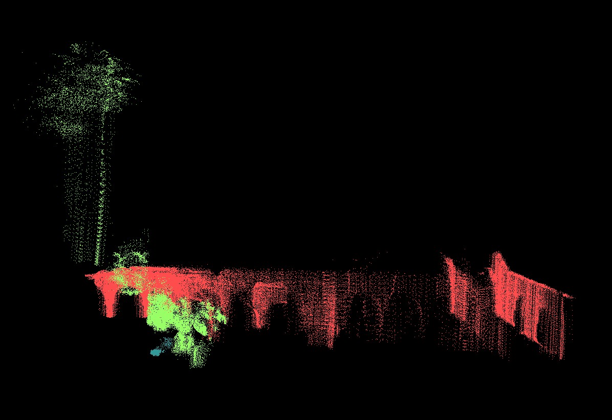
Below are the images of the labeled portion of the test set:

Labeled test image (180K points)

SVM

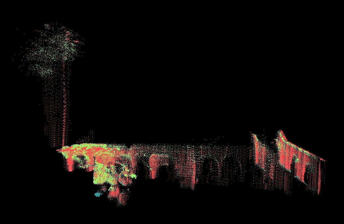Voted-SVM

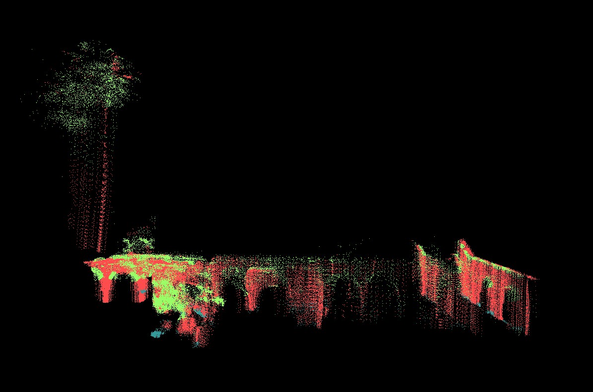AMN