 |
 |
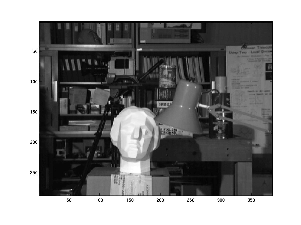
Left Image |
Right Image |
| |
|
Left Image |
Right Image |
 |
Disparity Map |
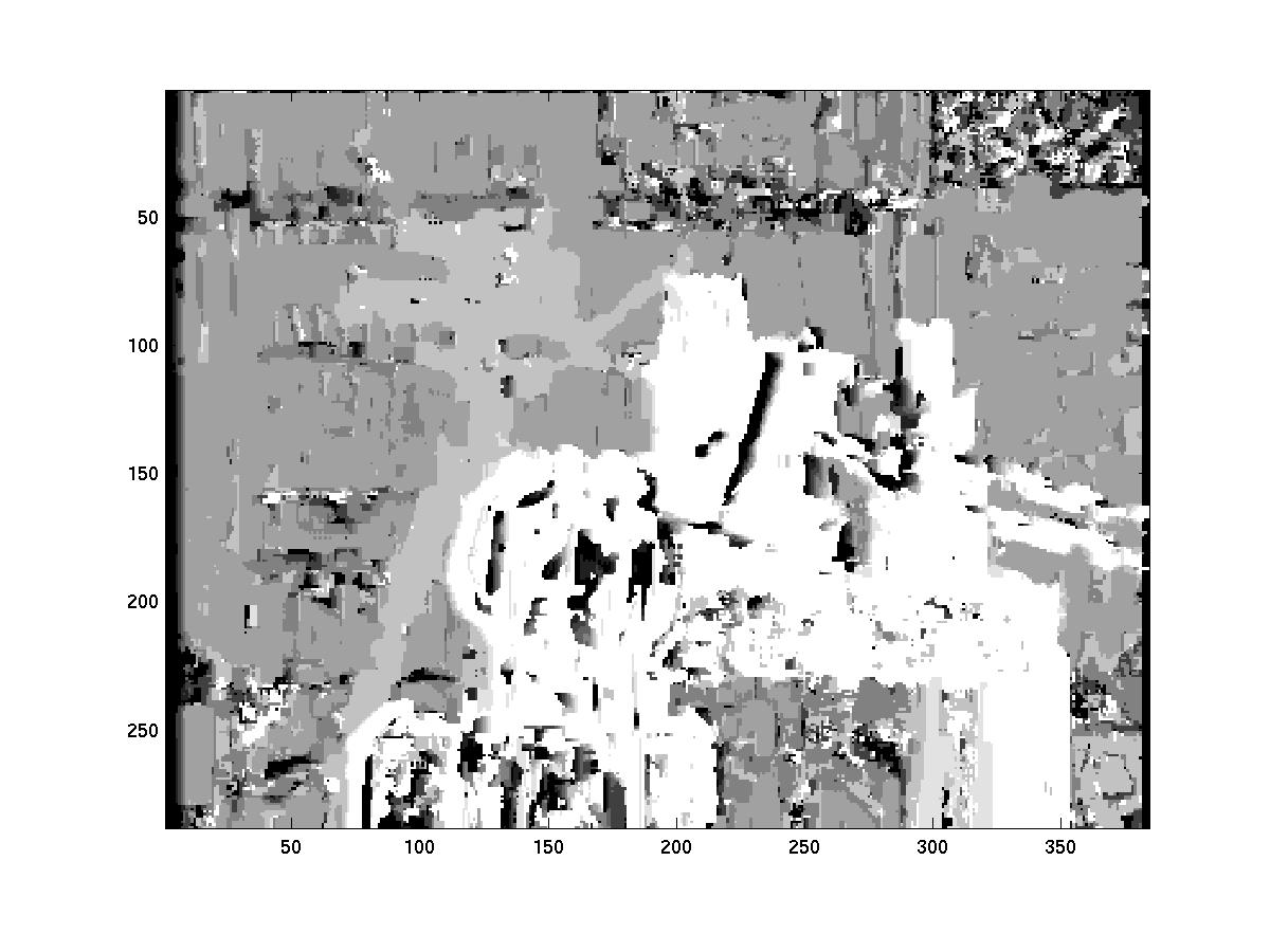
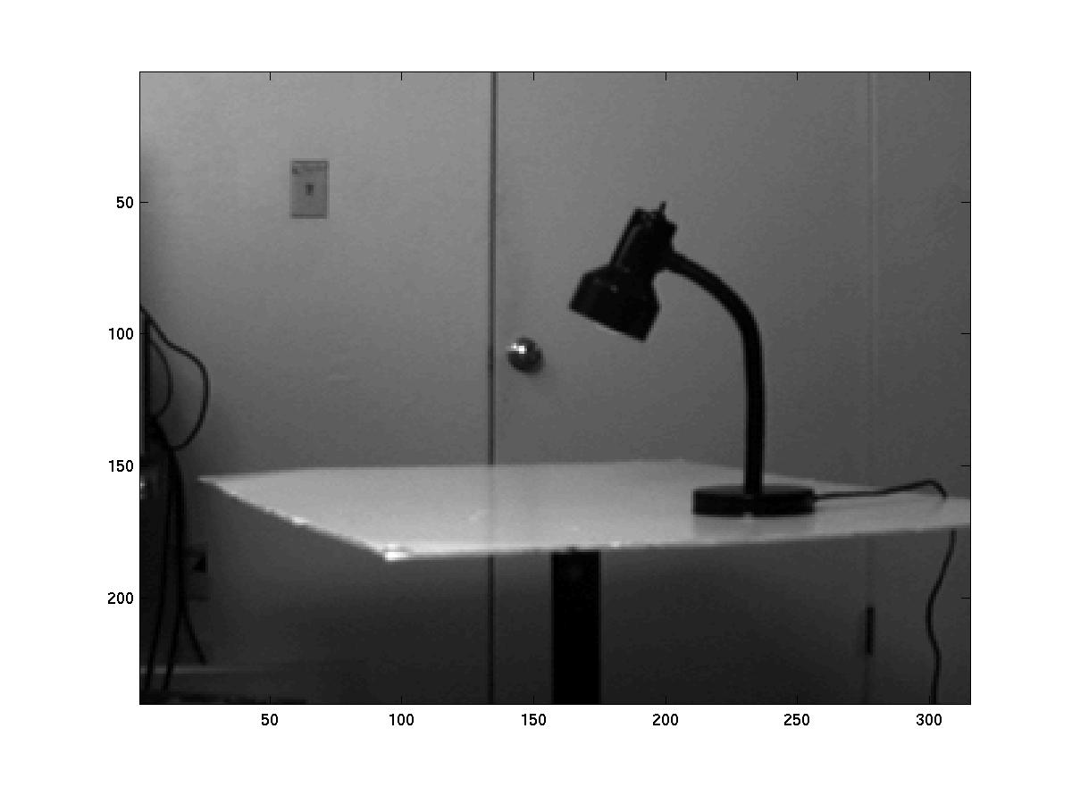
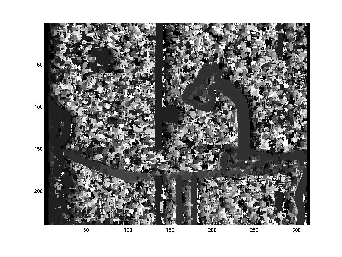
Observe that the lamp and the bust are too close for the current disparity limit. More often than not, the maximum disparity (i.e. 6) gives the lowest error for such cases so that most of these are colored white. However, at times, the error given by a lower disparity (say 0) would be lower than the error from high disparity (say 6) so that low disparity is chosen for that region. This is especially true of regions where there isn't too much intensity variation and its easy for the algorithm to get confused.
| |
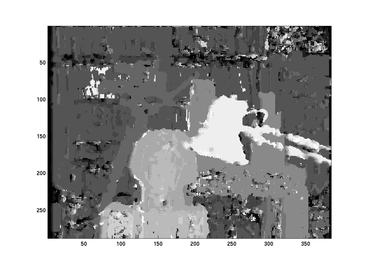 |
SSD | SAD |
 |
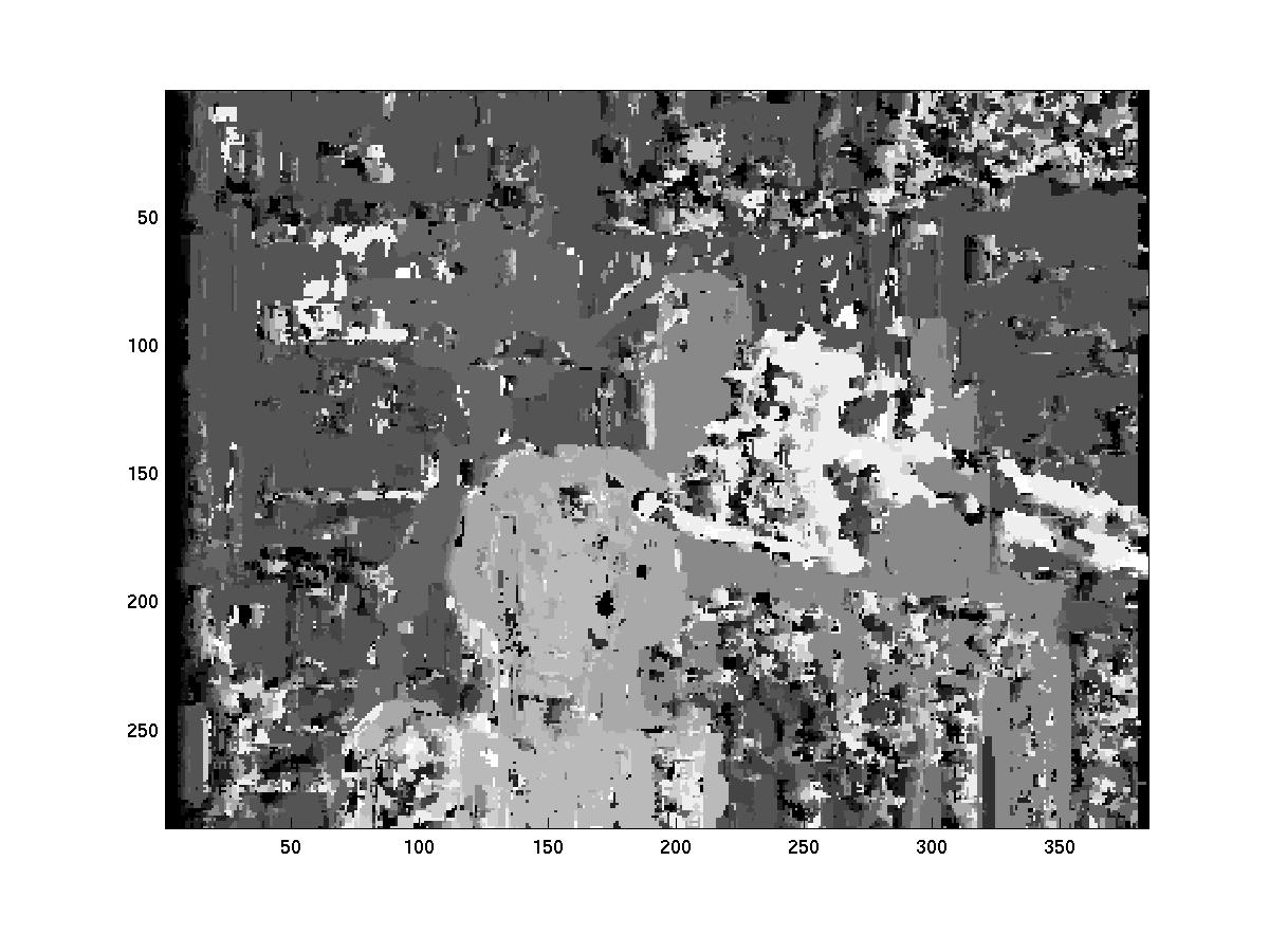 |
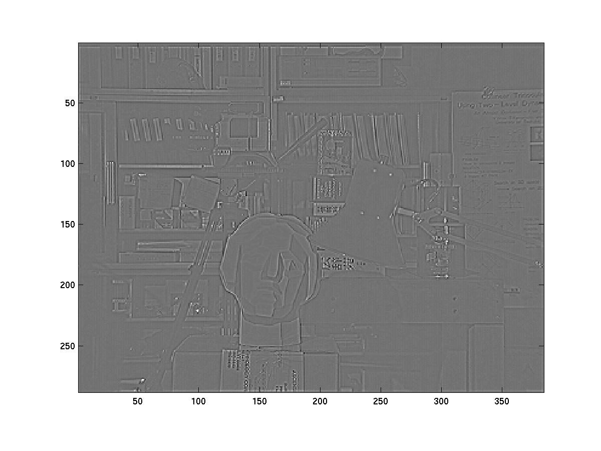
Left Image after Laplacian of Gaussian |
The disparity map of filtered image |
 |
 |
Left Image |
Right Image |
 |
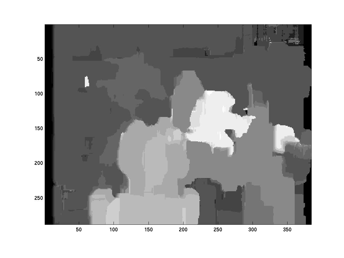
Disparity Map |
We felt that the Graph Cuts + Occlusion algo (ranked 2, number 4) was better. The edges were much crisp and the whole disparity map seemed to be free of noise. Moreover, regions of uniform intensity were very well handled. Obviously, the criteria to determine which algorithm is better are not only subjective (to the human being evaluating) but the criteria will differ for different sorts of cases. Dynamic programming seems to be introducing a lot of horizontal streaks in the disparity map. The realtime algorithm is ranked 12 in the given set.