Whether we're aware of it or not, computer vision is everywhere in our daily lives. For one, filtered photos are ubiquitous in our social media feeds, news articles, magazines, books—everywhere! Turns out, if you think of images as functions mapping locations in images to pixel values, then filters are just systems that form a new, and preferably enhanced, image from a combination of the original image's pixel values.

Images as Functions

To better understand the inherent properties of images and the technical procedure used to manipulate and process them, we can think of an image, which is comprised of individual pixels, as a function, f. Each pixel also has its own value. For a grayscale image, each pixel would have an intensity between 0 and 255, with 0 being black and 255 being white. f(x,y) would then give the intensity of the image at pixel position (x,y), assuming it is defined over a rectangle, with a finite range: f: [a,b] x [c,d] → [0, 255].

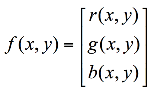
A color image is just a simple extension of this. f(x,y) is now a vector of three values instead of one. Using an RGB image as an example, the colors are constructed from a combination of Red, Green, and Blue (RGB). Therefore, each pixel of the image has three channels and is represented as a 1x3 vector. Since the three colors have integer values from 0 to 255, there are a total of 256*256*256 = 16,777,216 combinations or color choices.

An image, then, can be represented as a matrix of pixel values.

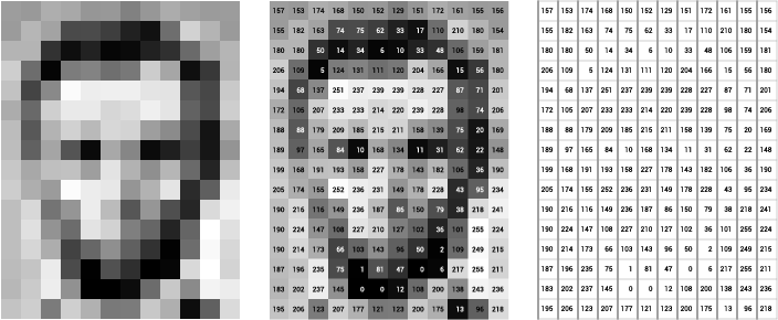
Image Processing

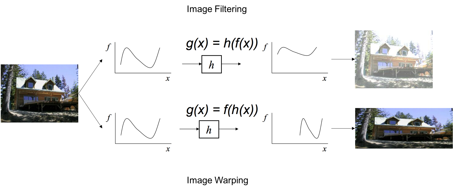
There are two main types of image processing: image filtering and image warping. Image filtering changes the range (i.e. the pixel values) of an image, so the colors of the image are altered without changing the pixel positions, while image warping changes the domain (i.e. the pixel positions) of an image, where points are mapped to other points without changing the colors.

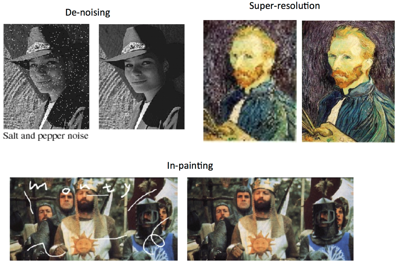
We will examine more closely image filtering. The goal of using filters is to modify or enhance image properties and/or to extract valuable information from the pictures such as edges, corners, and blobs. Here are some examples of what applying filters can do to make images more visually appealing.

Two commonly implemented filters are the moving average filter and the image segmentation filter.

The moving average filter replaces each pixel with the average pixel value of it and a neighborhood window of adjacent pixels. The effect is a more smooth image with sharp features removed.

If we used a 3x3 neighboring window:

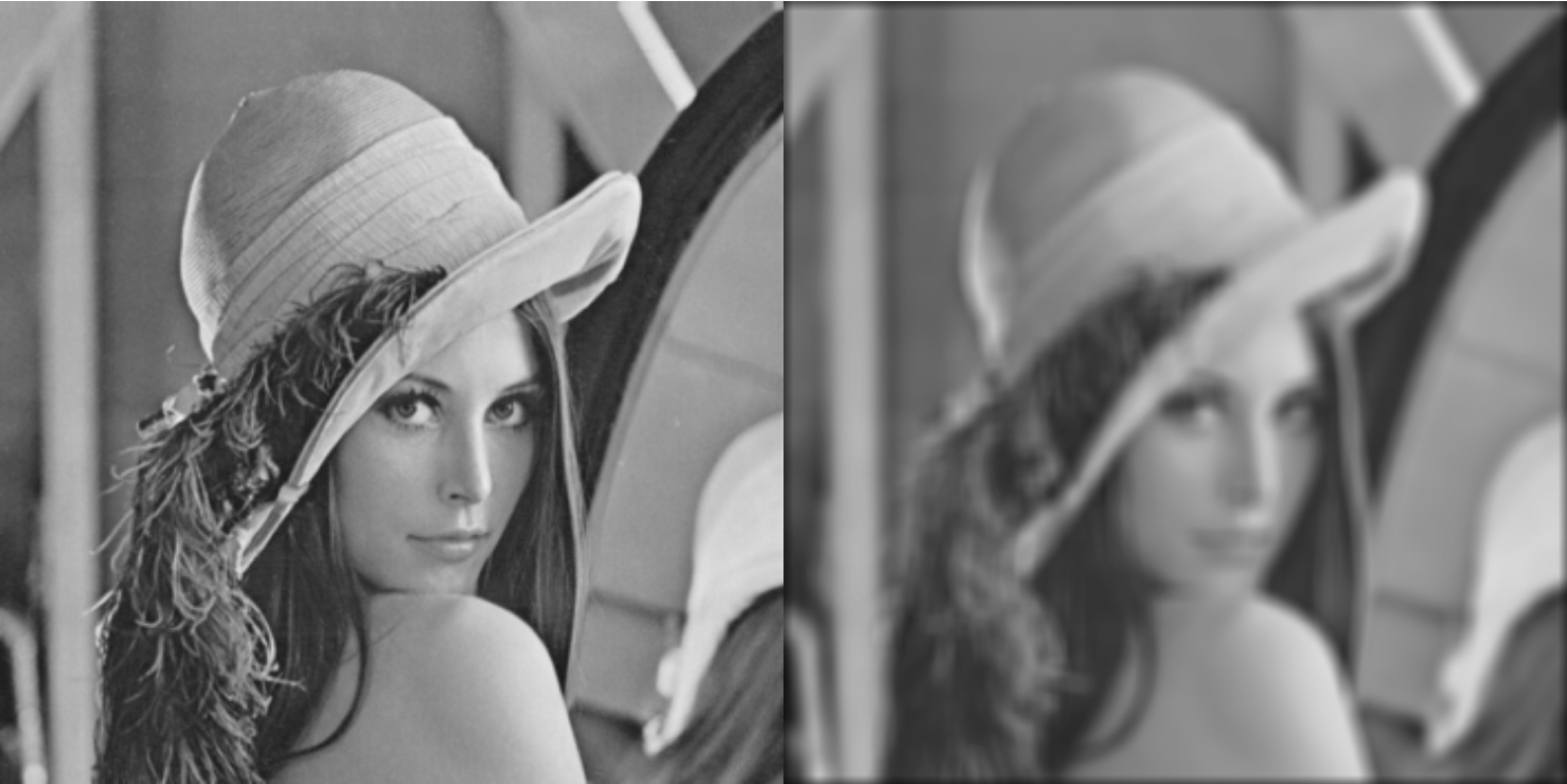
*Often times, applying these filters, as seen with the moving average, blurring, and sharpening filters, will produce unwanted artifacts along the edges of the images. To rid of these artifacts, zero padding, edge value replication, mirror extension, or other methods can be used.

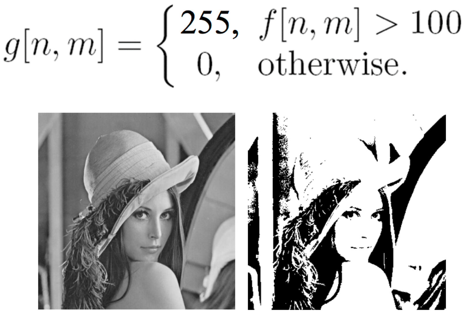
Image segmentation is the partitioning of an image into regions where the pixels have similar attributes, so the image is represented in a more simplified manner, and so we can then identify objects and boundaries more easily. There are multiple ways, which will be discussed in detail in Tutorial 3, to perform segmentation. Here, we will look at one simple way it can be implemented based on thresholding. In this example, all pixels with an intensity greater than 100 are replaced with a white pixel (intensity 255) and all others are replaced with a black pixel (intensity 0).

2D Convolution

The mathematics for many filters can be expressed in a principal manner using 2D convolution, such as smoothing and sharpening images and detecting edges. Convolution in 2D operates on two images, with one functioning as the input image and the other, called the kernel, serving as a filter. It expresses the amount overlap of one function as it is shifted over another function, as the output image is produced by sliding the kernel over the input image.

For a more formal definition of convolution, click here.

Let's look at some examples:

No change:

Shifted right by one pixel:

Blurred (you already saw this above):

Here's a fancier one that is a combination of two filters:

Sharpening filter:

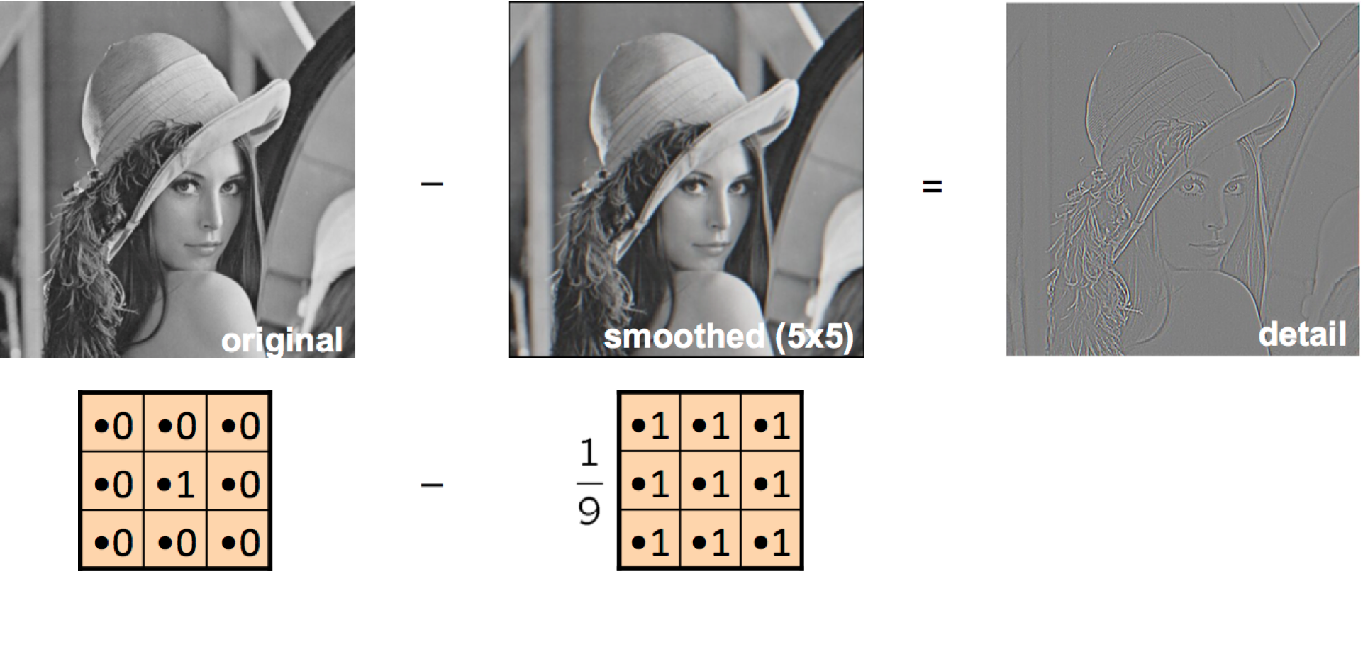
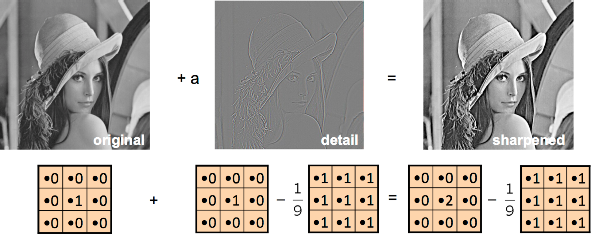
A sharpening filter can be broken down into two steps: It takes a smoothed image, subtracts it from the original image to obtain the "details" of the image, and adds the "details" to the original image.

Step 1: Original - Smoothed = "Details"

Step 2: Original + "Details" = Sharpened

Result:

Correlation

While a convolution is a filtering operation, correlation measures the similarity of two signals, comparing them as they are shifted by one another. When two signals match, the correlation result is maximized.

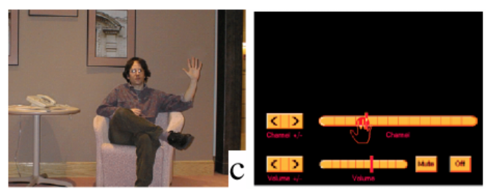
One application is is a vision system for using a hand to remotely control a TV. Template matching, based on correlation, is used to determine the hand position of the user to switch channels, increase or decrease volume, etc.

Edge Detection

In computer vision, edges are sudden discontinuities in an image, which can arise from surface normal, surface color, depth, illumination, or other discontinuities. Edges are important for two main reasons. 1) Most semantic and shape information can be deduced from them, so we can perform object recognition and analyze perspectives and geometry of an image. 2) They are a more compact representation than pixels.

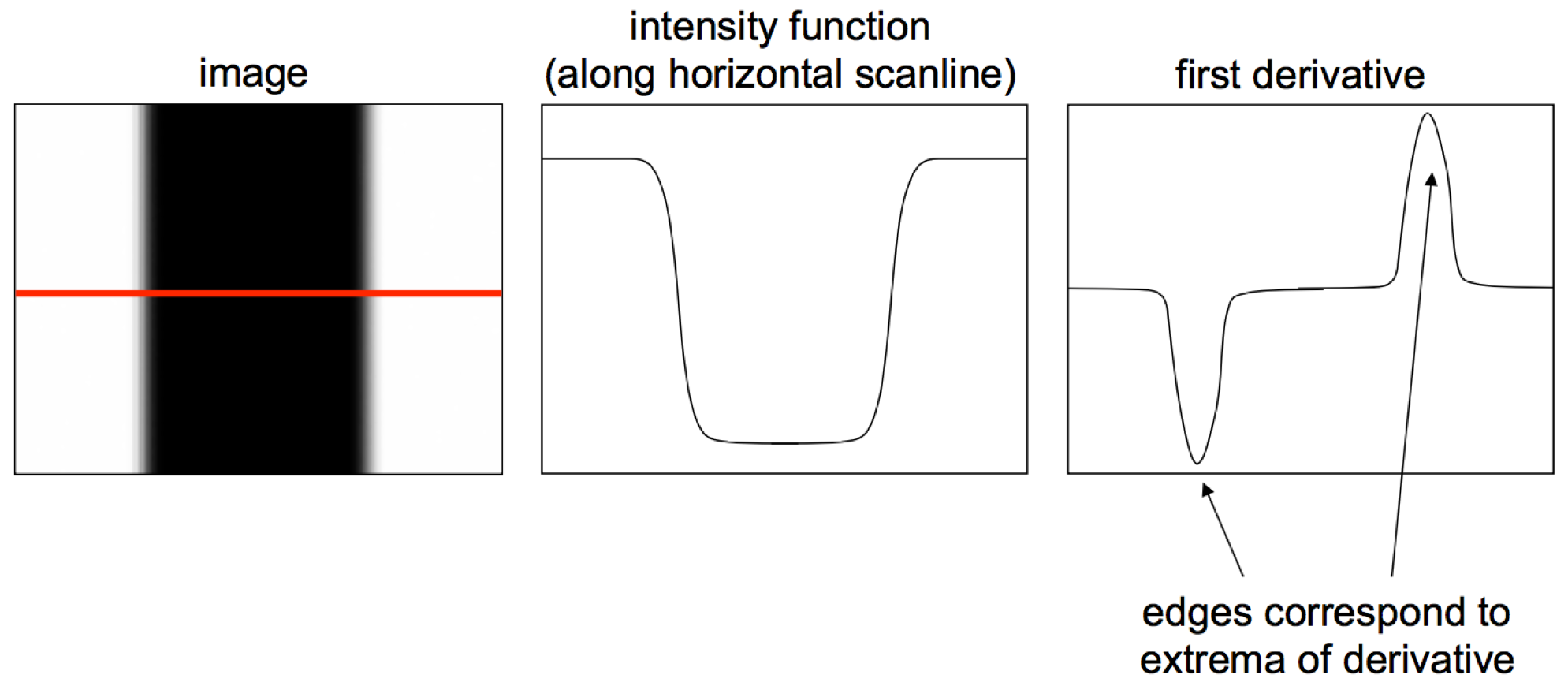
We can pinpoint where edges occur from an image's intensity profile along a row or column of the image. Wherever there is a rapid change in the intensity function indicates an edge, as seen where the function's first derivative has a local extrema.

An image gradient, which is a generalization of the concept of derivative to more than one dimension, points in the direction where intensity increases the most. If the gradient is ∇f = [^δf⁄_δx,^δf⁄_δy], then the gradient direction would be θ = tan^-1(^δf⁄_δy/^δf⁄_δx), and the edge strength would be the gradient magnitude: ||∇f|| = √(δf/δx)2+(δf/δy)2.

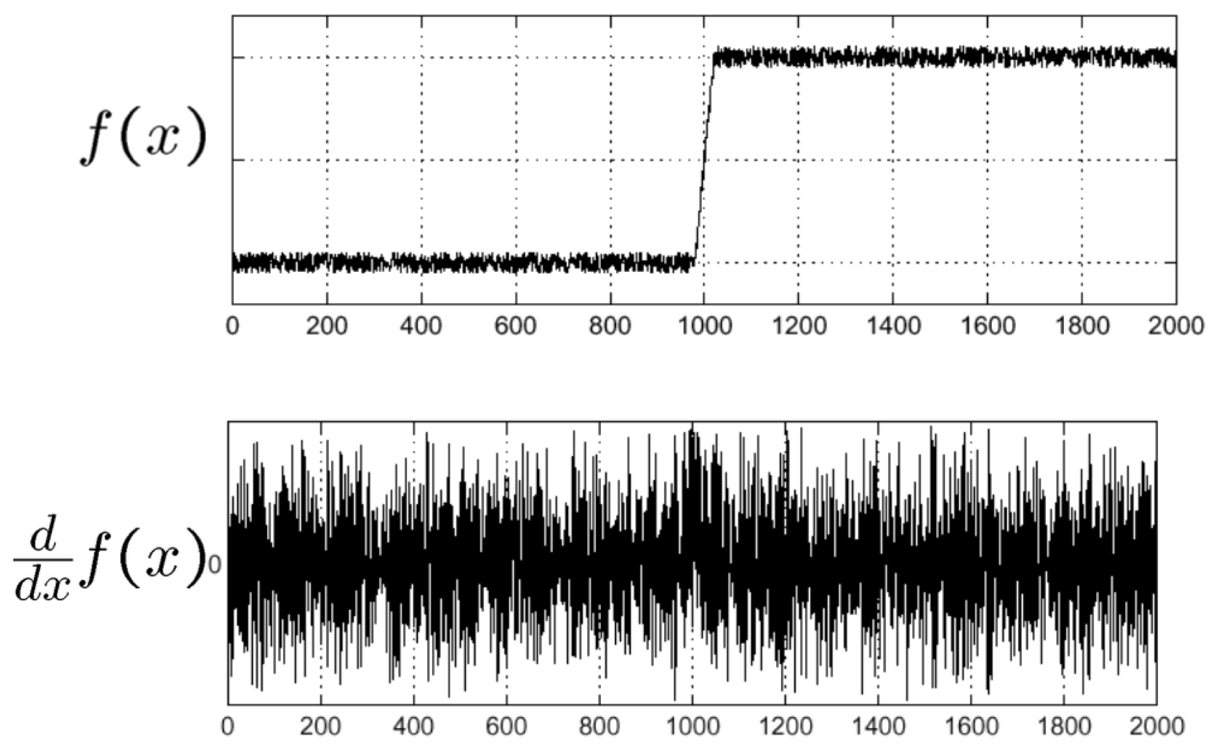
However, plotting the pixel intensities often results in noise, making it impossible to identify where an edge is by only taking the first derivative of the function.

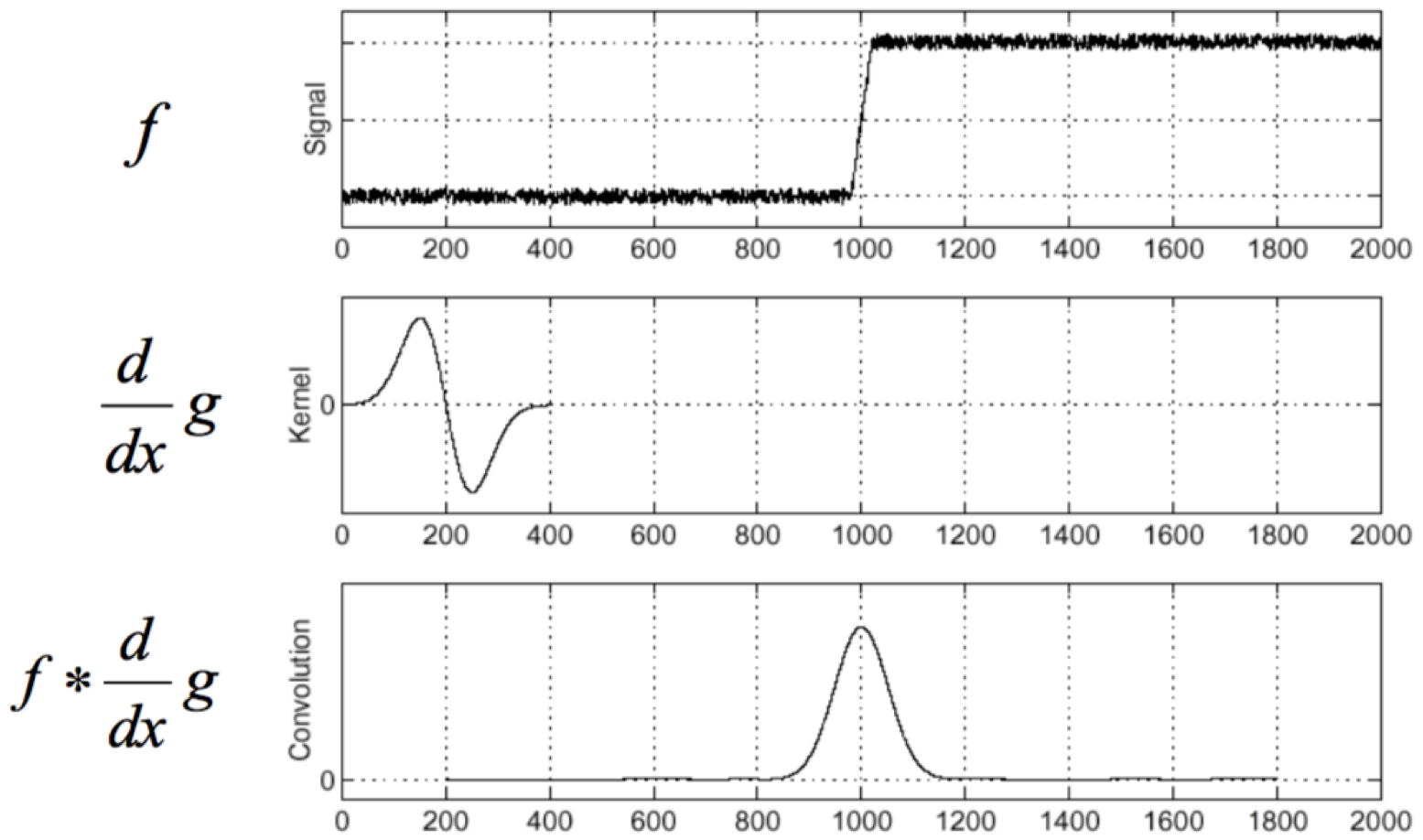
If we apply a filter that is a derivative of a Gaussian function, we can eliminate the image noise and effectively locate edges.

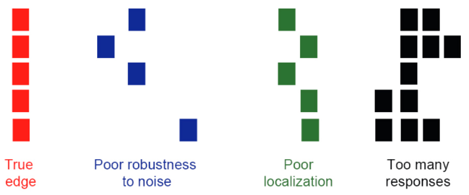
Building off of this procedure, we can design an edge detector. The optimal edge detector must be accurate, minimizing the number of false positives and false negatives; have precise localization, pinpointing edges at the positions where they actually occur; and have single response, ensuring that only one edge is found where there only is one edge.

The Canny edge detector is arguably the most commonly used edge detector in the field. It detects edges by:

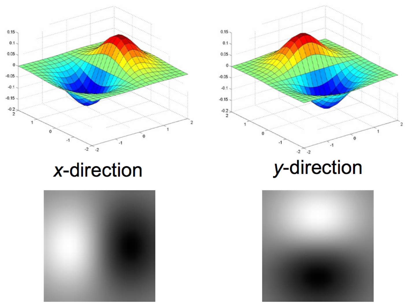
1. Applying the x and y derivatives of a Gaussian filter to the image to eliminate noise, improve localization, and have single response.



2. Finding the magnitude and orientation of the gradient at each pixel.
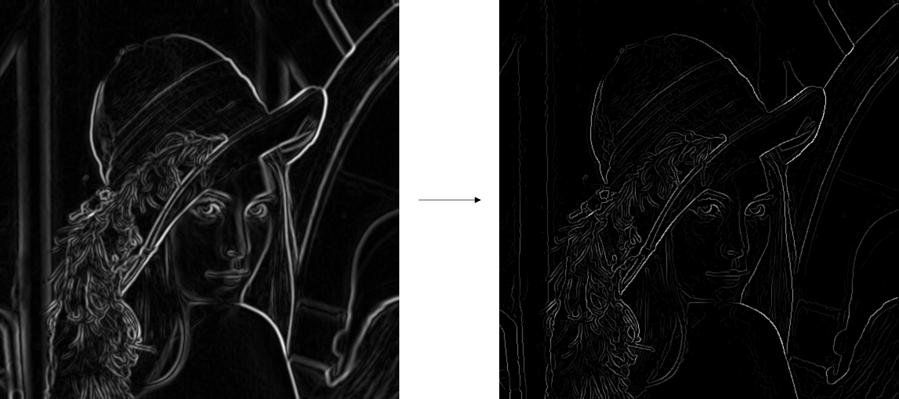
3. Performing non-maximum suppression, which thins the edges down to a single pixel in width, since the extracted edge from the gradient after step 2 would be quite blurry and since there can only be one accurate response.



4. Thresholding and linking, also known as hysteresis, to create connected edges. The steps are to 1. determine the weak and strong edge pixels by defining a low and a high threshold, respectively, and to 2. link the edge curves with the high threshold first to start with the strong edge pixels, continuing the curves with the low threshold.

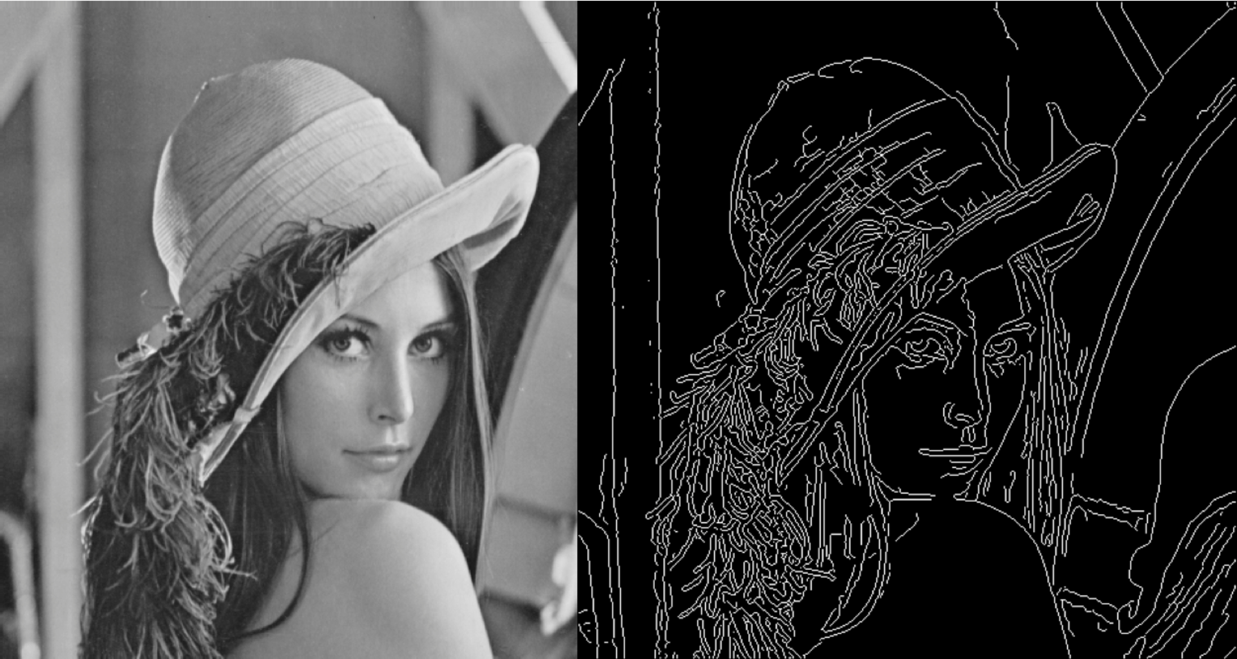
Final result:

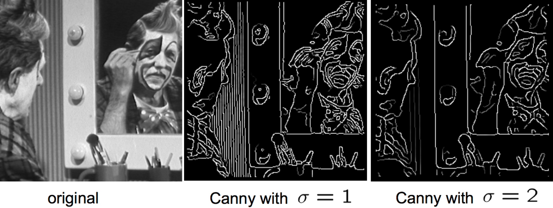
The Gaussian kernel size, σ, also affects the edges detected. If σ is large, the more obvious, defining edges of the picture are retrieved. Conversely, if σ is small, the finer edges are picked out as well.

To read more about the Canny edge detector, click here.

RANSAC: RANdom SAmple Consensus

Line fitting is important in edge detection since many objects are characterized by straight lines. However, edge detection does not always suffice since there can be extra edge points, muddling up which model would be the best, missing parts of lines, and noise. Thus, Fischler and Bolles developed the RANSAC algorithm, which determines a best fit line given a data set and avoids the effect of outliers by finding inliers. Given a scatterplot and a certain threshold, RANSAC randomly selects a sample of points, counts the number of inliers within the threshold, and repeats this process until the maximum number of inliers is hit.

You can learn more about RANSAC here.