ORL Images (examples.orl_images)
In this example of image processing we consider the image problem presented in [Hoyer2004].
We used the ORL face database composed of 400 images of size 112 x 92. There are 40 persons, 10 images per each person. The images were taken at different times, lighting and facial expressions. The faces are in an upright position in frontal view, with a slight left-right rotation. In example we performed factorization on reduced face images by constructing a matrix of shape 2576 (pixels) x 400 (faces) and on original face images by constructing a matrix of shape 10304 (pixels) x 400 (faces). To avoid too large values, the data matrix is divided by 100. Indeed, this division does not has any major impact on performance of the MF methods.
Note
The ORL face images database used in this example is included in the datasets and does not need to be
downloaded. However, download links are listed in the datasets. To run the example, the ORL face images
must exist in the ORL_faces directory under datasets.
We experimented with the Standard NMF - Euclidean, LSNMF and PSMF factorization methods to learn the basis images from the ORL database. The number of bases is 25. In [Lee1999] Lee and Seung showed that Standard NMF (Euclidean or divergence) found a parts-based representation when trained on face images from CBCL database. However, applying NMF to the ORL data set, in which images are not as well aligned, a global decomposition emerges. To compare, this example applies different MF methods to the face images data set. Applying MF methods with sparseness constraint, namely PSMF, the resulting bases are not global, but instead give spatially localized representations, as can be seen from the figure. Similar conclusions are published in [Hoyer2004]. Setting a high sparseness value for the basis images results in a local representation.
Note
It is worth noting that sparseness constraints do not always lead to local solutions. Global solutions can be obtained by forcing low sparseness on basis matrix and high sparseness on coefficient matrix - forcing each coefficient to represent as much of the image as possible.
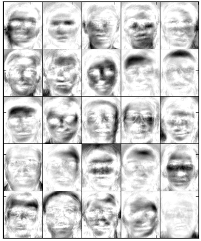
Basis images of LSNMF obtained after 500 iterations on original face images. The bases trained by LSNMF are additive but not spatially localized for representation of faces. Random VCol initialization algorithm is used. The number of subiterations for solving subproblems in LSNMF is a important issues. However, we stick to default and use 10 subiterations in this example.
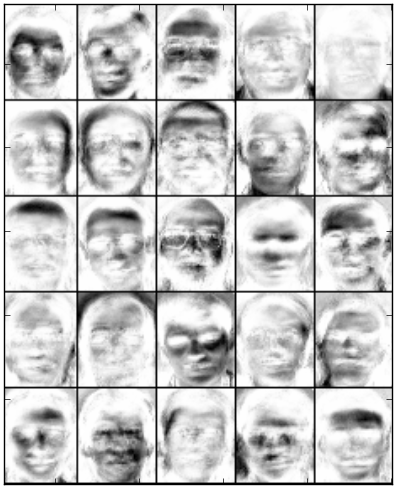
Basis images of NMF - Euclidean obtained after 200 iterations on reduced face images. The images show that the bases trained by NMF are additive but not spatially localized for representation of faces. The Euclidean distance of NMF estimate from target matrix is 33283.360. Random VCol initialization algorithm is used.
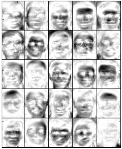
Basis images of LSNMF obtained after 200 iterations on reduced face images. The bases trained by LSNMF are additive. The Euclidean distance of LSNMF estimate from target matrix is 29631.784 and projected gradient norm, which is used as objective function in LSNMF is 7.9. Random VCol initialization algorithm is used. In LSNMF there is parameter beta, we set is to 0.1. Beta is the rate of reducing the step size to satisfy the sufficient decrease condition. Smaller beta reduces the step size aggressively but may result in step size that is too small and the cost per iteration is thus higher.
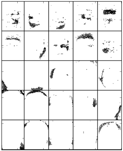
Basis images of PSMF obtained after 5 iterations on reduced face images and with set prior parameter to 5. The bases trained from PSMF are both additive and spatially localized for representing faces. By setting prior to 5, in PSMF the basis matrix is found under structural sparseness constraint that each row contains at most 5 non zero entries. This means, each row vector of target data matrix is explained by linear combination of at most 5 factors. Because we passed prior as scalar and not list, uniform prior is taken, reflecting no prior knowledge on the distribution.
To run the example simply type:
python orl_images.py
or call the module’s function:
import nimfa.examples
nimfa.examples.orl_images.run()
Note
This example uses matplotlib library for producing visual interpretation of basis vectors. It uses PIL
library for displaying face images.
-
nimfa.examples.orl_images.factorize(V)¶ Perform LSNMF factorization on the ORL faces data matrix.
Return basis and mixture matrices of the fitted factorization model.
Parameters: V (numpy.matrix) – The ORL faces data matrix.
-
nimfa.examples.orl_images.plot(W)¶ Plot basis vectors.
Parameters: W (numpy.matrix) – Basis matrix of the fitted factorization model.
-
nimfa.examples.orl_images.preprocess(V)¶ Preprocess ORL faces data matrix as Stan Li, et. al.
Return normalized and preprocessed data matrix.
Parameters: V (numpy.matrix) – The ORL faces data matrix.
-
nimfa.examples.orl_images.read()¶ Read face image data from the ORL database. The matrix’s shape is 2576 (pixels) x 400 (faces).
Step through each subject and each image. Reduce the size of the images by a factor of 0.5.
Return the ORL faces data matrix.
-
nimfa.examples.orl_images.run()¶ Run LSNMF on ORL faces data set.
