Introduction
Tokens are the basic units of information in Large Language Models (LLMs). It is a natural idea to replicate the success of LLMs in the vision domain by designing visual tokens. There have been a tons of attempts to learn visual tokens, or latents if you prefer, from different perspectivesA very nice blog by Dr. Sander Dieleman: Latents.. In this post, I would like to focus on a specific dimension: quantization. The concept of quantization dates back to the early 1980s when Robert M. Gray used it in signal processingRobert M. Gray, "Vector quantization." IEEE ASSP Magazine, Vol: 1, Issue: 2 (1986): 4-29.. A recent resurgent approach in the deep learning community is VQVAE, which uses a Variational Autoencoder (VAE) with a vector quantizer (VQ) bottleneck to learn the visual tokens. However, VQ is notoriously hard to train and scales poorly with a large codebook size. As a result, we end up in a paradox: we know the visual information carries much more data than language in quantity and diversityHuman language conveys information at a speed of at most 100 bits per second while the brain receives visual input at $10^6$ bits per seconds; However, the commonly used visual vocabulary size is much smaller than the language vocabulary sizesTypical values for visual vocabularies are around 1,204 to 16,384 (e.g., 8,192 in LVM and 16,384 in LlamaGen) whereas language vocabularies easily exceed 100,000 tokens (e.g., 199,997 in GPT-4o and 129,280 in DeepSeek-R1).. This paradox has stood long due to the quantization bottleneckThe word "bottleneck" is a pun. :P.
This post will review a few recent progresses on quantization methods. I will first review VQ: the basics, the challenges, and the remedies. Then I will focus on a family of quantization methods which I call non-parametric quantization (NPQ). I will provide a unified formulation from the perspective of lattice codes and reinterpret entropy regularization terms in NPQ as a lattice relocation problem. This later leads to a family of densest sphere-packing lattices, which features simplicity, efficiency, scalability, and effectiveness with provable guarantees. The Venn diagram below summarizes the concepts and methods to be covered in this post.
Click on the dots to explore different quantization methods and their relationships.
Vector Quantization
I will first review the basic idea of VQ and the training challenges. Let's consider a single image as input for simplicity $\mathbf{\mathit{I}} \in \mathbb{R}^{H \times W \times 3}$. The VQVAE uses an encoder-decoder (denoted by $\mathcal{E}$ and $\mathcal{G}$) pair to learn the visual tokens. A quantizer is placed in between.

Illustration of VQVAE. Figure is copied from Zhao et al. ICLR 2025.
$$ \mathbf{\mathit{I}} \xrightarrow[\text{encoder}]{\mathcal{E}(\cdot)} \mathbf{\mathit{Z}}\in \mathbb{R}^{\left(\frac{H}{p}\times\frac{W}{p}\right)\times d} \xrightarrow[\text{quantizer}]{\mathcal{Q}_\mathit{VQ}(\cdot)} \mathbf{\mathit{\hat{Z}}}\in \mathbb{R}^{\left(\frac{H}{p}\times\frac{W}{p}\right)\times d} \xrightarrow[\text{decoder}]{\mathcal{G}(\cdot)} \mathbf{\mathit{\hat{I}}} $$
Vector quantization maps a continuous vector $\mathbf{z} \in \mathbb{R}^d$ to the nearest codeword in a discrete codebook $\mathcal{C} = \{\mathbf{c}_1, \mathbf{c}_2, \ldots, \mathbf{c}_K\}$:$$\text{VQ}(\mathbf{z}) = \arg\min_{\mathbf{c}_k \in \mathcal{C}} \|\mathbf{z} - \mathbf{c}_k\|_2$$
The entire model ($\mathcal{E}$, $\mathcal{G}$, and $\mathcal{Q}$) is end-to-end trainable using gradient approximation methods such as straight-through estimator (STE).
$$ \mathbf{\hat{z}} = \mathrm{STE}(q(\mathbf{z})) = \mathbf{z} + \mathrm{stop}\mbox{-}\mathrm{gradient}(q(\mathbf{z}) - \mathbf{z}), \quad \frac{\partial \mathbf{\hat{z}}}{\partial \mathbf{z}} = I. $$
Challenges
Huh et al. comprehensively investigated the trainability of VQ networks in their ICML 2023 paper. To summarize, the codebook gradient sparsity and the asymmetric nature of the commitment loss results in a covariate shift (see figure below) between the codebook and the embedding distribution. The gradient approximation error caused by STE further exacerbates the issue.
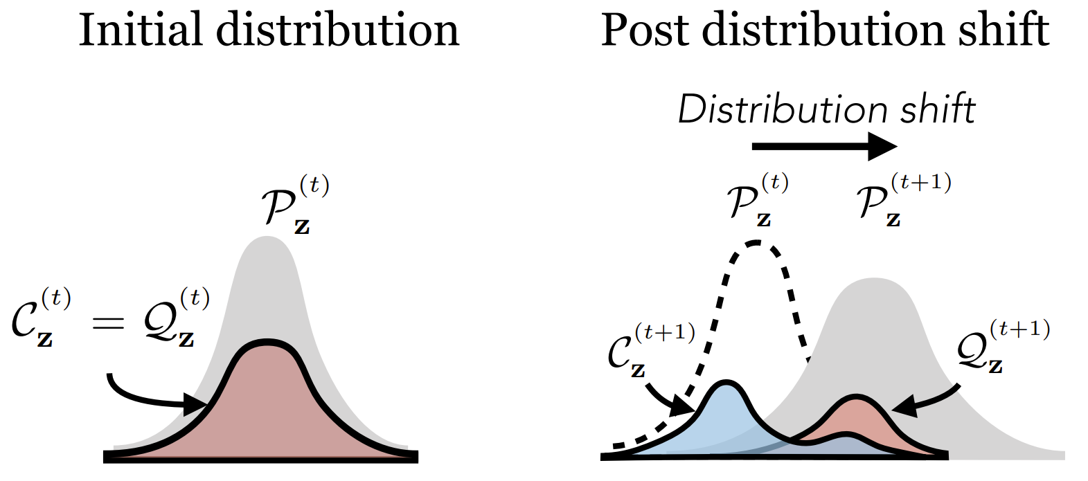
Illustration of codebook covariate shift. The figure is copied from Huh et al. ICML 2023.
Remedies
Knowing the causes, we can now devise remedies. The first is to align the codebook distribution and the embedding distribution. This can be achieved by: (1) Rewaking the dead codewords with replacement or online clustering, and (2) Re-parameterizing the code vectors for better alignment using affine transformations or meta-learning. The second is to find better approximations for the gradients. I enumerate the representative methods below:
Rotary trick. Intead of an identity mapping in STE, the rotary trick rotates the gradients with respect to the support codevectors.$$ \mathbf{\hat{z}} = \mathrm{stop}\mbox{-}\mathrm{gradient}\left(\frac{|| \mathbf{\hat{z}} ||}{|| \mathbf{z} ||} \mathbf{\mathit{R}} \right) \mathbf{z}, \quad \frac{\partial \mathbf{\hat{z}}}{\partial \mathbf{z}} = \frac{|| \mathbf{\hat{z}} ||}{|| \mathbf{z} ||} \mathbf{\mathit{R}}, $$
where $ \mathrm{\mathit{R}} $ is the rotation matrix computed with Householder matrix reflections, i.e., $ \mathrm{\mathit{R}} = \mathrm{\mathit{I}} - 2 rr^\top + 2 \frac{\mathrm{\hat{z}}}{\|\mathrm{\hat{z}}\|} \frac{\mathrm{z}}{\|\mathrm{z}\|}^\top $ ($ r = \frac{\mathrm{z} + \mathrm{\hat{z}}}{\|\mathrm{z} + \mathrm{\hat{z}}\|} $).Gumbel softmax.
$ \mathbf{l} = \mathrm{Linear}(\mathbf{z}) \in \mathbb{R}^K , \quad \mathbf{g} \sim \mathrm{Gumbel}(0, 1) $ Or equivalently, $ g = -\log(-\log(u)) $ where $ u \sim \mathrm{Uniform}(0, 1) $. $$ \mathbf{y} = \mathrm{softmax}(\frac{\mathbf{l} + \mathbf{g}}{\tau}) = [ \cdots, \frac{e^{(l_k + g_k) / \tau}}{\sum_{i=k'}^K e^{(l_{k'} + g_{k'}) / \tau}}, \cdots ]^\top $$ $$ \mathbf{\hat{z}} = \mathbf{y}^\top\mathbf{\mathit{C}} $$
Index Backpropagation. IB can be written in a very similar way to Gumbel softmax. The difference is that (1) it uses the dot product between the embedding and the codevectors to get the logits rather than a learnable linear layer, (2) it adds no Gumbel bias, and (3) it uses a one-hot encoding of the indices instead of a softmax to get the quantized output.
$$ \mathbf{l} = [\mathbf{z}^\top \mathbf{c}_1, \mathbf{z}^\top \mathbf{c}_2, \ldots, \mathbf{z}^\top \mathbf{c}_K]^\top $$ $$ \mathbf{y} = \mathrm{stop}\mbox{-}\mathrm{gradient}(\mathrm{one}\mbox{-}\mathrm{hot}(\mathbf{l}) - \mathrm{softmax}(\mathbf{l}) ) + \mathrm{softmax}(\mathbf{l}) $$ $$ \mathbf{\hat{z}} = \mathbf{y}^\top\mathbf{\mathit{C}} $$
Non-Parametric Quantization
The basic idea behind the so-called non-parametric quantization (NPQ) method is simple: Now that learning two seprate sets of parameters in a synchronous pace is hard, why don't we just learn one of them and keep the other fixed? We opt to fix the codebook and only learn the encoder-decoderThe community has known so well how to design and train a good encoder-decoder given the spent GPU years.. Once the codebook is fixed, the quantized output can be easily computed using basic arithmetic operations (sign, fused multiply-add, etc.).
Known NPQ Methods
Lookup-free quantization (LFQ). Yu et al. introduced the implicit codebook representation using binary codes, i.e., $ \mathbf{C} = \{ \pm1 \}^d $., where its best quantizer a binary quantization (or sign function), $ \mathcal{Q}_\textit{LFQ}(z) = \mathrm{sign}(z) $.
$$ \mathbf{z} \xrightarrow[\text{quantize}]{\mathcal{Q}_\mathit{LFQ}(\cdot)} \hat{\mathbf{z}} = \mathrm{sign}(\mathbf{z}). $$
Binary Spherical Quantization (BSQ). In BSQ, both the embedding and the codevectors are on a unit $d$-hypersphere, i.e., $ \mathbf{C} = \{ \pm\frac{1}{\sqrt{d}} \}^d $, where the best quantizer is sign function up to a scalar multiplier.
$$ \mathbf{z} \xrightarrow[\text{normalize}]{f(\cdot)} \bar{\mathbf{z}} = \frac{\mathbf{z}}{\|\mathbf{z}\|} \xrightarrow[\text{quantize}]{\mathcal{Q}_\mathit{BSQ}(\cdot)} \hat{\mathbf{z}} = \frac{1}{\sqrt{d}} \mathrm{sign}(\bar{\mathbf{z}}). $$
Finite Scalar Quantization (FSQ) is similar to LFQ but extends the codebook to multiple values per dimension i.e. $\prod_{i=1}^d \{0, \cdots , \pm \lfloor \frac{L_i}{2} \rfloor \}$.From now on, I will assume $L_i = L$ for all $i$ for simplicity. This assumption eases the lattice formulation.
$$ \mathbf{z} \xrightarrow[\text{bound}]{f(\cdot)} \bar{\mathbf{z}} = \lfloor \frac{L}{2} \rfloor \tanh(\mathbf{z}) \xrightarrow[\text{quantize}]{\mathcal{Q}_\mathit{FSQ}(\cdot)} \hat{\mathbf{z}} = \mathrm{round}(\bar{\mathbf{z}}). $$
Discussions on LFQ, BSQ, and FSQ. Both LFQ and BSQ require an entropy regularization term to encourage high code utilization.
$$ \mathcal{L}_\mathrm{entropy} = \mathbb{E} \left[ H[q(\mathbf{z})] \right] - \gamma H\left[ \mathbb{E} \left[ q(\mathbf{z}) \right] \right], $$ where $q(\mathbf{z})\approx \hat{q}(\mathbf{c} | \mathbf{z}) = \frac{\exp(-\tau (\mathbf{c}-\mathbf{z})^2)}{\sum_{\mathbf{c} \in \mathbf{C}} \exp(-\tau (\mathbf{c}-\mathbf{z})^2)}$ is a soft quantization approximation.
LFQ is easiest to implement, but the computational cost for entropy increases exponentially. BSQ provides an efficient approximation with a guaranteed bound, but still suffers from codebook collapse without regularization. FSQ does not need such complex regularization, but the way to obtain the number of levels per channel $L$ (or $(L_1, \cdots, L_d)$) is somewhat heuristic.Visualizing NPQ
I use Voronoi diagrams to illustrate how different NPQ methods partition the latent spaceWe show the hexagonal lattice here for illustrative purpose. A more formal introduction will be given shortly.. Each codevector defines a region (Voronoi cell) where all points in that region are quantized to the same codevector. By looking at the right arrow showing the quantization error $ \mathbf{\hat{z}} - \mathbf{z} $, we can easily see how STE deviates from the true "gradient" of the quantization function.
Comparison of Voronoi partitions. (Top-Left) LFQ with 4 corner codevectors, $ (\pm 1, \pm1) $; (Top-Right) BSQ with 4 codevectors, $ (\pm 1/\sqrt{2}, \pm1/\sqrt{2}) $; (Bottom-Left) FSQ with grid-like codevectors, $ \{\pm 2, \pm1, 0\} \times \{\pm 2, \pm1, 0\} $; (Bottom-Right) Hexagonal spherical lattice (which is the densest packing lattice at $d=2$) with 6 codevectors $ \{ (\cos(\theta), \sin(\theta)) | \theta = \frac{(1+2N)\pi}{6}, N\in\{0,1,2,3,4,5\} \} $.
Lattice-based Codes
We want to find a common language to describe all these NPQ methods. Looking at the gometric landscape above, we observe that the codevectors are arranged in a regular grid, also known as lattice.
Lattice. A $d$-dimensional lattice is defined by a discrete set of points in $\mathbb{R}^d$ that constitutes a group. In particular, the set is translated such that it includes the origin. Mathematically, it is written as: $$ {\Lambda}_d = \{ {\lambda} \in \mathbb{R}^{d} | \lambda = \mathbf{G} \mathbf{b} \}, \mathbf{G} = \begin{bmatrix} | & | & & | \\ \mathbf{g}_1 & \mathbf{g}_2 & \cdots & \mathbf{g}_d \\ | & | & & | \end{bmatrix}, $$ where $\mathbf{G} \in \mathbb{R}^{d\times d}$ is called the generator matrix, comprising $d$ generator vectors $\mathbf{g}_i$ in columns, and $\mathbf{b}\in\mathbb{Z}^d$. $ {\Lambda}_d $ by its definition has infinite elements. In practice, we often consider a finite subset of $ {\Lambda}_d $ by including some constraints. $$ {\Lambda}_d = \{ {\lambda} \in \mathbb{R}^{d} | \lambda = \mathbf{G} \mathbf{b}, \mathbf{b}\in\mathbb{Z}^d, \underbrace{f(\lambda) = c_1, h(\lambda) \leq c_2 }_{\text{constraints}} \}. $$ Particularly, spherical lattice codes refer to a family with a constant squared norm, i.e., $$ {\Lambda}_{d,m} = \{ {\lambda} \in \mathbb{R}^{d} | \lambda = \mathbf{G} \mathbf{b}, \mathbf{b}\in\mathbb{Z}^d, \underbrace{\| \lambda\|^2 = m}_\text{length constraint} \}. $$ Besides, we define the quantizer associated with $ \Lambda $ by $ \mathcal{Q}_\Lambda(\mathbf{z}) = \arg\min_{t \in \Lambda} \| \mathbf{z} - t \| $, which offers a bridge between lattice code and vector quantization.
NPQ as Lattice Codes
From the perspective of the lattice-based codes, the above NPQ variants can be described in the same language with different instantiations of the generator matrix and constraints. I will provide a summary in the Grand Tableau section and leave more details in the technical report.
Entropy regularization as lattice relocation
The entropy regularization term heavily used in NPQ (LFQ and BSQ) can be interpreted from the perspective of lattice coding too. Let me first write it down again:
$$ \mathcal{L}_\mathrm{entropy} = \underbrace{\mathbb{E} \left[ H[q(\mathbf{z})] \right]}_{\text{clustering}} ~ \underbrace{- \gamma H\left[ \mathbb{E} \left[ q(\mathbf{z}) \right] \right]}_{\text{diversity}}. $$
The first term minimizes the entropy of the distribution that $\mathbf{z}$ is assigned to one of the codes. This means that every input should be close to one of the centroids instead of the decision boundary. This principle is known as clustering assumption.This becomes less of an issue when the codebook of interest is much larger nowadays, examplified by the fact that the optimal $\gamma$ is usually greater than 1.The second term is more important. It maximizes the entropy of the assignment probabilities averaged over the data, which favors class balance or diversity. Assuming that $\mathbf{z}$ has a uniform distribution over its input range, we can see that $ \mathbb{E}[q(\mathbf{z})] = P(q(\mathbf{z}) = \mathbf{c}_k ) = \int_{V_k} d\mathbf{z} = | V_k | $, which is the volume of the Voronoi region for the codevector $\mathbf{c}_k$. $H[\mathbb{E}[q(\mathbf{z})]]$ is maximized if all Voronoi cells have equal volumes.
It is easy to see that FSQ's codebook configuration indeed maximizes the entropy term implicitly, which explains why it can be trained without any regularization as reported in Mentzer et al.. In contrast, this does not hold for LFQ, because the unbounded input range breaks the uniform distribution assumption. This does not hold for BSQ either, but the anaylsis is slightly different as the input embeddings are projected on a hypersphere beforehand.
Spherical lattices and hypersphere packing
The Voronoi regions on the hypersphere shells can take arbitrary shapes. For simplicity, we create two surrogate problems where we approximate the Voronoi shells with the regions partitioned by various hyperballs.
Illustration of varied radii configuration for sphere packing but in the case of $\mathbb{R}^2$. (Left) Voronoi partition of 5 points in the plane; (Right) Circles with varied radii such that they are close to each other.
The first surrogate problem studies how to place $N$ $d$-dimensional balls with varied radii, where $N$ is the cardinality of the lattice in which we are interested. Under this settings, the entropy maximization term corresponds to finding the most dispersive configuration to relocate the balls, in other words, maximizing the minimum distance between any pair of pointsThis is also known as the Tammes' problem when $d=3$., or more formally,
$$ \max_{\mathbf{c}_1,\cdots,\mathbf{c}_N \in \mathbb{R}^{d-1}} \underbrace{\min_{1 \leq j < k \leq N } d(\mathbf{c}_j, \mathbf{c}_k) }_{\delta_\min (N)}. $$
We solve the problem by generalizing the Fibonacci lattice to $d$-dimensional hyperspheres. Simulations show that the Fibonacci lattice, denoted as $\mathbb{F}_d(N)$, achieves near-optimal performance at low $d$ (i.e., $d=3$) but becomes suboptimal (only comparable to the random projection baseline) when $d$ increases.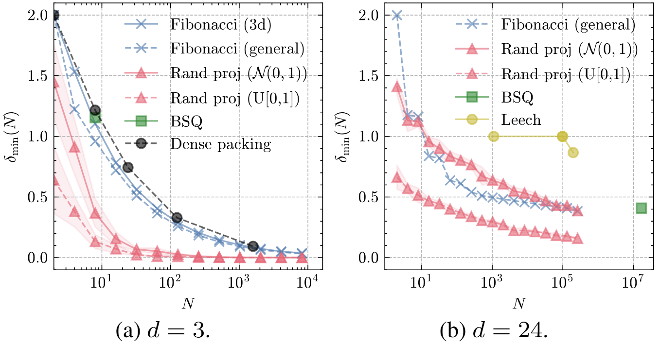
$\delta_\min (N)$ w.r.t. $N$ for different $d$. The figure is copied from Zhao et al. arXiv 2025.
Illustration of varied radii (left) and equal radii (right) configurations for sphere packing in $\mathbb{R}^2$. Note the empty space between the circles in the both figures.
The second surrogate problem assumes equal radii for all hyperspheres and find the densest sphere packingThe packing density is defined by the ratio of the volume of the hyperspheres to the volume of the containing hyperballs.. The general solution is still an open problem, but the best known results in dimensions 1 to 8, 12, 16, and 24 are summarized below, where $\mathbb{Z}$ to $\mathbb{E}_8$ and $\Lambda_{24}$ have been proved optimal among all lattices. For example, $ \mathbb{A}_2 $ is also known as the hexagonal lattice, where the spherical shells have already been shown in the bottom right of .
| 1 | 2 | 3 | 4 | 5 | 6 | 7 | 8 | 12 | 16 | 24 | |
|---|---|---|---|---|---|---|---|---|---|---|---|
| denset packing | $\mathbb{Z}$ | $\mathbb{A}_2$ | $\mathbb{A}_3$ | $\mathbb{D}_4$ | $\mathbb{D}_5$ | $\mathbb{E}_6$ | $\mathbb{E}_7$ | $\mathbb{E}_8$ | $\mathbb{K}_{12}$ | $\Lambda_{16}$ | $\Lambda_{24}$ |
The best known densest sphere packing in different dimensions. The table is adapted from Table 1.1 in Conway and Sloane.
We pay particular attention to the Leech lattice $\Lambda_{24}$, which is the densest sphere packing in 24 dimensions. Normalizing the 196,560 vectors in the first shell to unit length results in the Spherical Leech Quantization ($\Lambda_{24}$-SQ) codes.Simplified loss combo
Thanks to the dense sphere packing principle, the entropy regularization term is gone. Thanks to the non-parametric nature, the commitment loss is gone too. This leads to the simplified loss combo: Mean Absolute Error (MAE) + perceptual loss + GAN loss. I would also like to argue that this trio is not reducible any more because they directly optimize the downstream metrics that we care about. These metrics are somewhat "orthogonal" to each other from the information theoretical perspective.
| MAE | Perceptual loss | GAN loss | |
|---|---|---|---|
| Loss formulation | $ d(\mathbf{X}, \mathbf{\hat{X}}) $ | $ d(VGG(\mathbf{X}), VGG(\mathbf{\hat{X}})) $ | $ \log{D(\mathbf{X})} - \log{(1-D(\mathbf{\hat{X}}))} $ $\Rightarrow JSD(p_\mathbf{X} || p_\mathbf{\hat{X}}) $ |
| Optimizing metric | PSNR, SSIM | LPIPS | FID |
| Information theoretical language | $\mathbb{E}[d(\mathbf{X}, \mathbf{\hat{X}})]$ pixel-level similarity |
$\mathbb{E}[d(VGG(\mathbf{X}), VGG(\mathbf{\hat{X}}))]$ feature-level similarity |
$div(\mathcal{N}(\mu_\mathbf{X}, \Sigma_\mathbf{X}) || \mathcal{N}(\mu_\mathbf{\hat{X}}, \Sigma_\mathbf{\hat{X}}))$ distributional similarity(divergence) |
The Grand Tableau
Now that I have introduced all the NPQ methods, I can compare them in a grand table. It contains definitions (e.g. generator matrix), properties (e.g. vocabulary size), and concepts important for analyzing the quantization methods (e.g., quantization error).
Comparison of non-parametric quantization methods.
Results
We showcase some key results in this section. For more results, please refer to the technical report.Non-Parametric vs. Learnable
We compare $\Lambda_{24}$-SQ with BSQ and Random Projection VQ on the ImageNet reconstruction task using the same ViT-based VQGAN architecture. We restrict the input resolution to $128 \times 128$, and the ViT is a standard ViT-S/8 model. The results are shown below, where $\Lambda_{24}$-SQ consistently outperforms BSQ and Random Projection VQ across all metrics. The rightmost two bars are learnable VQ using $\Lambda_{24}$-SQ and random projection codebook as initialization. We can see that the non-parametric quantization methods are competitive (<2% gap) to the learnable counterparts.
Comparison of $\Lambda_{24}$-SQ ($d^*=\log(196560)=17.58$) and others on ImageNet reconstruction. Higher is better for PSNR and SSIM; lower is better for LPIPS and rFID.
Compression
We compare the effectiveness of compression of $\Lambda_{24}$-SQ with other methods on the Kodak datasethttps://r0k.us/graphics/kodak/.. The methods include traditional codecs, including JPEG2000 and WebP, and tokenizer-based approaches, including MAGVIT2 and BSQ. Note that the rate-distortion tradeoff can be further improved (~25% less bitrate) by training an unconditional AR model for arithmetic coding.
Comparison of compression performance. (Left) PSNR vs. bpp; (Right) MS-SSIM vs. bpp.
Epilogue
To sum up, this post discussed a family of quantization methods called non-parametric quantization (NPQ). The spherical constraints ensures a bounded gradient approximation error caused by the non-differentiable nature of quantization. The principle of dense sphere packing implicitly maintains the diversity of the latents. The resulting $\Lambda_{24}$-SQ achieves the optimal trade-off between bitrate and reconstruction quality compared to existing methods, with a simplified training recipe.
Open questions
Continuous latents vs. discrete tokens? It is a long-standing debate in the community whether to use continuous latents or discrete tokens. Some may argue that continuous latents lead to better reconstruction quality but our analysis suggests that this is at the cost of higher bitrateE.g., each element of a continuous latent in the VAE tokenizer should be counted as 16 bits since the checkpoint is stored in FP16. In contrast, each element of a BSQ token takes only 1 bit. Generally speaking, a discrete token takes $\log_2(|\mathcal{C}|)$ bits, where $|\mathcal{C}|$ is the codebook size.. From this perspective, the debate between continuous latents and discrete tokens should be reconsidered under the rate-distortion tradeoff framework.
What does the latent really mean? Rather than asking if we should use continuous latents or discrete tokens, we should ask how the latent looks like and what the latent means. We have seen some progress made in the interpretability of LLMs and would love to expect more studies in vision models too.
Do we really need visual tokenization? I have recently noticed a resurgence of interest in pixel-based visual generation, which natually raises this question. It is an appealing idea to build generative models directly on the raw data in those domains "where tokenizer are difficult to obtain". Our efforts, however, aim to make the tokenizer easier to build. Visual tokenization is still needed in many aspects. One is compression, where we are interested in representing the data in some "units", measured by bits. Another is multimodal modeling - building a stronger visual tokenizer is likely to benefit multimodal models consistentlyMany other factors come into play. I hope another post will cover this topic in more detail soonish..
Acknowledgements
I would like to thank the following people, institutes, and funding sources for supporting this work.- My PhD advisor Philipp Krähenbühl.
- My Postdoc advisor Ehsan Adeli.
- Co-authors: Yuanjun Xiong🐻, Hanwen Jiang, Zhenlin Xu, and Chutong Yang.
- 2024-2025 NVIDIA Graduate Fellowship and UT Dean’s PFS for financial support.
- The NSF AI Institute for Foundations of Machine Learning (IFML) and Center for Generative AI (CGAI) for funding this research.
- Texas Advanced Computing Center (TACC) for providing computational resources.
- Lambda Inc. for compute credits.
References
The reference mentioned in this post is listed below. For a more comprehensive list, please refer to the here and there.- Van Den Oord, A., Vinyals, O. "Neural discrete representation learning." NeurIPS 2017.
- Bai, Y., et al. "Sequential modeling enables scalable learning for large vision models." CVPR 2024.
- Sun, P., et al. "Autoregressive model beats diffusion: Llama for scalable image generation." arXiv 2024.
- OpenAI. "GPT-4o System Card." https://openai.com/index/gpt-4o-system-card/.
- DeepSeek. "DeepSeek-R1 technical report." 2025.
- Mentzer, F., et al. "Finite scalar quantization: VQ-VAE made simple." ICLR 2024.
- Yu, L., et al. "Language model beats diffusion - tokenizer is key to visual generation." ICLR 2024.
- Zhao, Y., et al. "Image and video tokenization with binary spherical quantization." arXiv 2024.
- Zhao, Y., et al. "Spherical Leech Quantization for Visual Tokenization and Generation." arXiv 2025.
- Chiu, C., et al. "Self-supervised Learning with Random-projection Quantizer for Speech Recognition." ICML 2022.
- Bengio, Y., et al. "Estimating or propagating gradients through stochastic neurons for conditional computation." arXiv 2013.
- Łancucki, A., et al. "Robust training of vector quantized bottleneck models." IJCNN 2020.
- Zheng, C. and Vedaldi, A. "Online Clustered Codebook." CVPR 2023.
- Dhariwal, P., et al. "Jukebox: A Generative Model for Music." arXiv 2020.
- Huh, M., et al. "Straightening Out the Straight-Through Estimator: Overcoming Optimization Challenges in Vector Quantized Networks." ICML 2023.
- Qin, P. and Zhang, J. "Learning to Quantize for Training Vector-Quantized Networks." ICML 2025.
- Krause, A., et al. "Discriminative clustering by regularized information maximization." NeurIPS 2010.
- Grandvalet, Y. and Bengio, Y. "Semi-supervised learning by entropy minimization." NeurIPS 2004.
- Ericson, T. and Zinoviev, V. "Codes on Euclidean spheres." Elsevier 2001.
- Sloane, N. J. A., et al. "Spherical codes." URL: http://neilsloane.com/packings/, 2000.
- Tammes, P. M. L. "On the origin of number and arrangement of the places of exit on the surface of pollen-grains." Recueil des travaux botaniques néerlandais 1930.
- González, Á. "Measurement of areas on a sphere using fibonacci and latitude–longitude lattices." Mathematical geosciences 2010.
- Conway, J. H., and Sloane, N. J. A. "Sphere packings, lattices and groups." Springer Science & Business Media, 2013.
- Fifty, C., et al. "Restructuring vector quantization with the rotation trick." ICLR 2025.
- Jang, E., et al. "Categorical reparameterization with gumbel-softmax." ICLR 2017.
- Shi, F., et al. "Scalable image tokenization with index backpropagation quantization." ICCV 2025.
- Jansen, A., et al. "Coincidence, categorization, and consolidation: Learning to recognize sounds with minimal supervision." ICASSP 2020.
- Agustsson, E., et al. "Soft-to-hard vector quantization for end-to-end learning compressible representations." NeurIPS 2017.
- Blau, Y. and Michaeli, T., et al. "Rethinking Lossy Compression: The Rate-Distortion-Perception Tradeoff." ICML 2019.
- Dhariwah, P., and Nichol, A. "Diffusion models beat gans on image synthesis." NeurIPS 2021.
- Hoogeboom, E., et al. "Simpler diffusion (SiD2): 1.5 fid on imagenet512 with pixel-space diffusion." CVPR 2025.
- Wang, S., et al. "PixNerd: Pixel neural field diffusion." arXiv 2025.
- Li, T., and He, K. "Back to Basics: Let Denoising Generative Models Denoise." arXiv 2025.
- Shannon, C.E. "A mathematical theory of communication." Bell System Technical Journal 1948.
- Anthropic. "Scaling Monosemanticity: Extracting Interpretable Features from Claude 3 Sonnet." https://transformer-circuits.pub/2024/scaling-monosemanticity/index.html. 2024.
- Shannon, C.E. "Prediction and entropy of printed English." Bell System Technical Journal 1951.
- Koch, K. "How much the eye tells the brain." Current biology 2006.
- John Leech. "Notes on sphere packings." Canadian Journal of Mathematics, 19:251-267, 1967.
- Delétang, G., et al. "Learning to compress with neural arithmetic coders." ICLR 2024.