TL;DR
Want something better than \(k\)-means? Our state-of-the-art \(k\)-medoids algorithm from NeurIPS, BanditPAM, is now publicly available! \(\texttt{pip install banditpam}\) and you're good to go!
Like the \(k\)-means problem, the \(k\)-medoids problem is a clustering problem in which our objective is to partition a dataset into disjoint subsets. In \(k\)-medoids, however, we require that the cluster centers must be actual datapoints, which permits greater interpretability of the cluster centers. \(k\)-medoids also works better with arbitrary distance metrics, so your clustering can be more robust to outliers if you're using metrics like \(L_1\).
Despite these advantages, most people don't use \(k\)-medoids because prior algorithms were too slow. In our NeurIPS paper, BanditPAM, we sped up the best known algorithm from \(O(n^2)\) to \(O(n\text{log}n)\).
We've released our implementation, which is pip-installable. It's written in C++ for speed and supports parallelization and intelligent caching, at no extra complexity to end users. Its interface also matches the \(\texttt{sklearn.cluster.KMeans}\) interface, so minimal changes are necessary to existing code.
Useful Links:
\(k\)-means vs. \(k\)-medoids
If you're an ML practitioner, you're probably familiar with the \(k\)-means problem. In fact, you may know some of the common algorithms for the \(k\)-means problem. You're much less likely, however, familiar with the \(k\)-medoids problem.
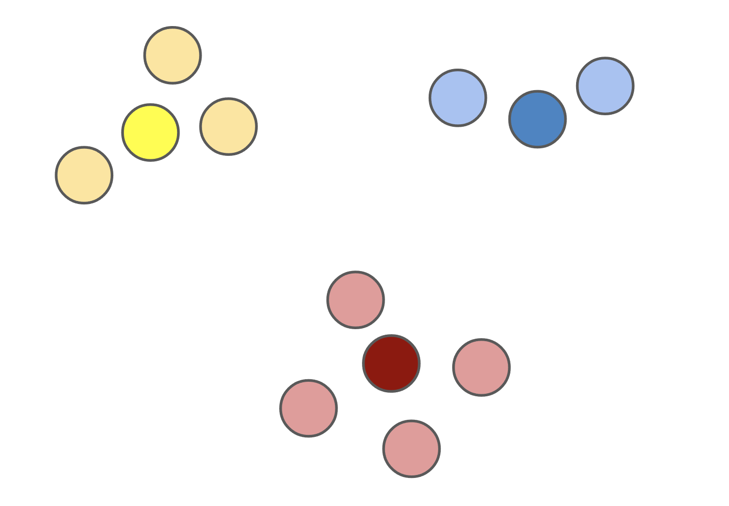
The \(k\)-medoids problem is a clustering problem similar to \(k\)-means. Given a dataset, we want to partition our dataset into subsets where the points in each cluster are closer to a single cluster center than all other \(k-1\) cluster centers. Unlike in \(k\)-means, however, the \(k\)-medoids problem requires cluster centers to be actual datapoints.
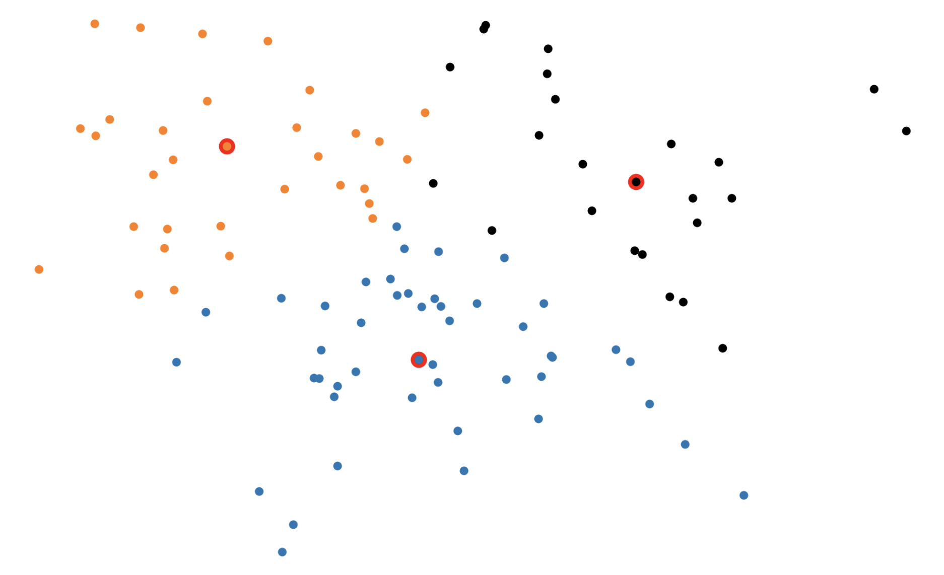
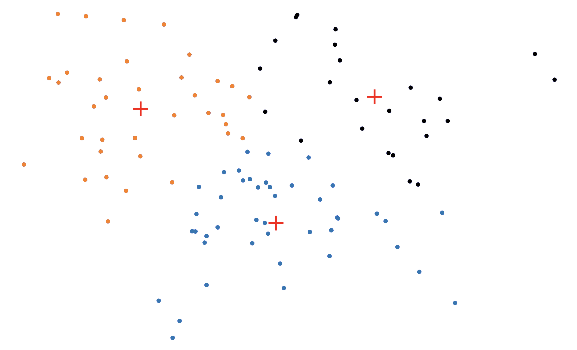
Figure 1: The \(k\)-medoids solution (left) forces the cluster centers to be actual datapoints. This solution is often different from the \(k\)-means solution (right).
The \(k\)-medoids problem has several advantages over \(k\)-means. By forcing the cluster centers -- dubbed the medoids -- to be actual datapoints, solutions tend to be more interpretable since you can determine exactly which datapoint is the cluster center for each cluster. When clustering images from the ImageNet dataset, for example, the mean of a solution to the \(k\)-means problem with \(k = 1\) is usually a nondescript blob (Figure 2, left), whereas the medoid of a corresponding solution to the \(k\)-medoids problem is an actual image (Figure 2, right).

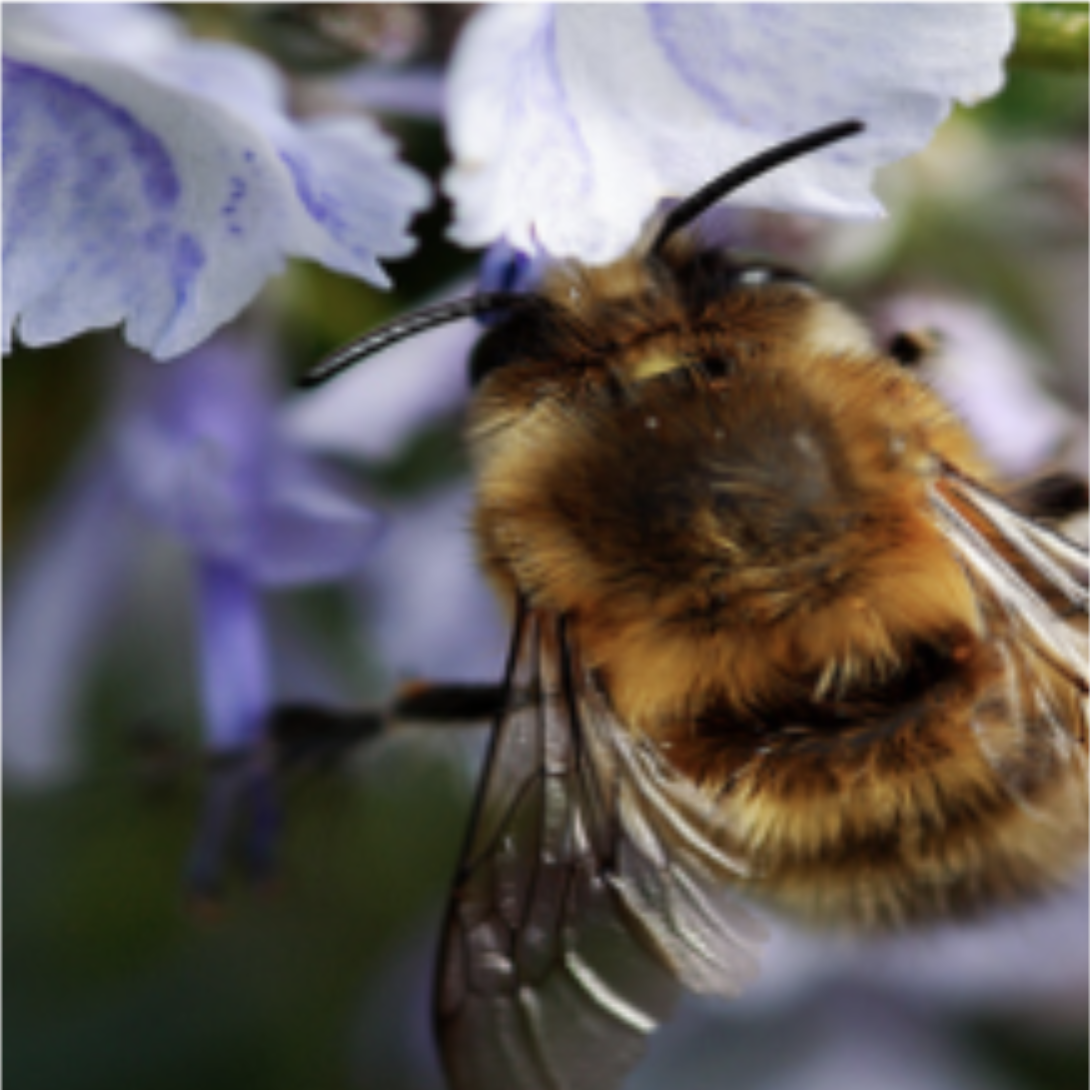
Figure 2: The cluster centers in \(k\)-means are often not easily interpretable, whereas they are actual datapoints in \(k\)-medoids. Shown are cluster centers for a subset of ImageNet with \(k = 1\) with \(k\)-means (left) and \(k\)-medoids (right). The mean of the dataset is the average per-pixel color, whereas the medoid is an image of a bee.
The \(k\)-medoids problem also supports arbitrary distance metrics, in contrast with \(k\)-means which usually requires \(L_2\) for efficiency. In fact, you're allowed to use any pairwise dissimilarity function with \(k\)-medoids -- your dissimilarity function need not even satisfy the properties of a metric. It can be asymmetric, negative, and violate the triangle inequality. In practice, allowing for arbitrary dissimilarity metrics enables the clustering of "exotic" objects like strings, natural language, trees, graphs, and more -- without needing to embed these objects in a vector space first.
The advantages of \(k\)-medoids don't stop there. Because the \(k\)-medoids problem supports arbitrary distance functions, the clustering can often be more robust to outliers if you're using robust distance metrics. The \(L_1\) metric, for example, is more robust to outliers than the \(L_2\) metric; in one dimension, the \(L_1\) minimizer is the median of your datapoints whereas the \(L_2\) minimizer is the mean.
Despite all of these advantages, \(k\)-means is much more widely used than \(k\)-medoids, largely due to its much more favorable runtime. The best \(k\)-means algorithms scale linearly in dataset size, i.e., have \(O(n)\) complexity, whereas, until now, the best \(k\)-medoids algorithms scaled quadratically in dataset size, i.e., had \(O(n^2)\) complexity.
In our NeurIPS paper, BanditPAM, we reduced the complexity of the best known \(k\)-medoids algorithm from \(O(n^2)\) to \(O(n\text{log}n)\). This complexity almost matches the complexity of standard \(k\)-means algorithms -- and now, you get all the benefits of \(k\)-medoids on top. We've also released a high-performance implementation of our algorithm written in C++ for speed but callable from Python via python bindings; \(\texttt{pip install banditpam}\) and you're ready to go! Our algorithm's interface matches that of \(\texttt{sklearn.cluster.KMeans}\) and can be used with a simple 2-line change. You can also implement your own distance metrics, interpret cluster centers, and cluster structured data!
BanditPAM: Almost Linear Time \(k\)-medoids Clustering via Multi-Armed Bandits
How does our algorithm, BanditPAM, work? Our claim is that we match the prior state-of-the-art solutions in clustering quality by recovering the exact same solution and reduce the complexity from \(O(n^2)\) to \(O(n\text{log}n)\). But is this reduction in complexity just "for free"?
To discuss BanditPAM, we first need to discuss its predecessor, the Partitioning Around Medoids (PAM) algorithm. The PAM algorithm, first proposed in 19901, is a greedy solution to the \(k\)-medoids problem. PAM is broken into two steps: the BUILD step and the SWAP step.
In the BUILD step, each of the \(k\) medoids is greedily initialized one by one. More concretely, PAM considers all possible datapoints as "candidate" medoids. For every candidate medoid, we compute the change in the overall loss if we were to add that candidate to the set of medoids, conditioned on the previously assigned medoids being fixed. This results in \(O(n^2)\) computational complexity since we need to compute every pairwise distance.
In the SWAP step, we consider all \(kn\) (medoid, non-medoid) pairs and the change in loss that would be induced if we were to swap the first element of the pair out of the medoid set in favor of the second. Again, this procedure incurs an \(O(n^2)\) time complexity (really \(O(kn^2))\).

Figure 3: The \(k\)-medoids algorithm in action. In the BUILD step, each medoid is assigned greedily, one by one. In the SWAP step, we consider swapping medoid assignments to see if we can lower the overall loss.
Our fundamental insight was that for each step of the PAM algorithm, we don't actually need to compute the distance from each point to all other \(n\) points. Instead, we can just sample these distances!
Consider, for example, the problem of assigning the first medoid at the beginning of the BUILD step. PAM would go through all \(n\) points and, for each point, compute its distance to every other point. We realized that for each candidate, we only needed to compute the distance to \(O(\text{log}n)\) other points. By intelligently choosing which distances to compute, we can save a lot of unnecessary computation. Formally, we reduce the problem of assigning the first medoid to a multi-armed bandit problem, as demonstrated in Figure 4. In multi-armed bandit problems, our objective is to identify the best action to take -- also referred to as the best arm to pull -- when actions are independent and have stochastic returns.
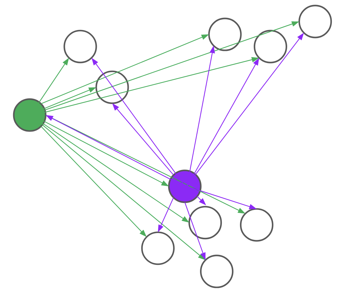
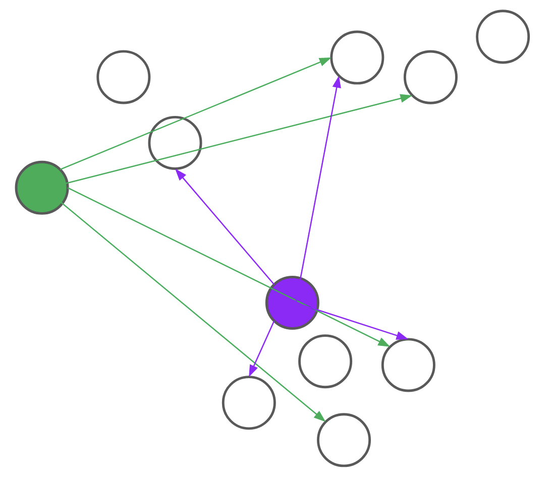
Figure 4: PAM (left) computes every pairwise distance for each candidate medoid. BanditPAM (right) only samples the pairwise distances. With just a few samples, we see that the purple point is a better candidate than the green point since the purple arrows are, on average, shorter than the green ones.
It turns out that all steps of the PAM algorithm can also be reduced to multi-armed bandit problems. In each part of the BUILD step, we still view each candidate datapoint as an arm. Now, however, pulling an arm corresponds to computing the induced change in loss for a random datapoint if we were to add the candidate to the set of medoids, conditioned on the previous medoids already being assigned. In each SWAP step, we view each (medoid, non-medoid) pair as an arm and pulling an arm corresponds to computing the induced change in loss on a random datapoint if we were to perform the swap. With these modifications, the original PAM algorithm is now reformulated as a sequence of best-arm identification problems. This reformulation reduces every step of the PAM algorithm from \(O(n^2)\) to \(O(nlogn)\).
Now, if you're familiar with multi-armed bandits, you might protest. Our algorithm is a randomized algorithm and can sometimes return an incorrect result. In the full paper, we show that the probability of getting a "wrong" answer is very small. In practice, this means that users of our algorithm don't have to worry and will almost always get the same answer as the original PAM algorithm.
The BanditPAM algorithm is an \(O(n\text{log}n)\) algorithm that matches prior state-of-the-art algorithms in clustering quality and almost matches the complexity of popular \(k\)-means algorithms. Want to try out BanditPAM? Run \(\texttt{pip3 install banditpam}\) and jump to our examples.

Figure 5: A formal proof that \(k\)-medoids is superior to \(k\)-means in every way.
Acknowledgments
This blog post is based on the paper: BanditPAM: Almost Linear Time \(k\)-medoids Clustering via Multi-Armed Bandits. NeurIPS 2021.
A special thanks to my collaborators on this project, Martin Jinye Zhang, James Mayclin, Sebastian Thrun, Chris Piech, and Ilan Shomorony, as well as the reviewers of this blog post, Drew A. Hudson and Sidd Karamcheti.
-
Kaufman, Leonard; Rousseeuw, Peter J. (1990-03-08), "Partitioning Around Medoids (Program PAM)", Wiley Series in Probability and Statistics, Hoboken, NJ, USA: John Wiley & Sons, Inc., pp. 68–125] ↩