The Compass Operator

vs.

The Canny Operator

Mark A. Ruzon

We have claimed that the compass operator out-performs the Canny operator, and shown convincing results that, at least in two examples, the compass operator does indeed do better. Although the two schemes appear to have little in common, we will show that, simply by rearranging the order of operations, Canny's edge detector is actually a special case of the compass operator.

How Canny's Edge Detector Works

In 1986 John Canny published a landmark paper in the IEEE Transactions on Pattern Analysis and Machine Intelligence that introduced what is currently the most popular edge detection algorithm. Canny derived, for a 1-D signal (we will restrict ourselves to greyscale images in one dimension for a while), a family of convolution filters, and then chose as his filter the derivative of a Gaussian, which was an approximation to one member of his family.

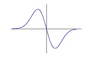
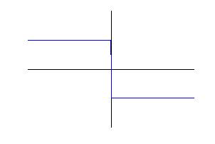
An edge is detected by placing the operator at a point in the signal (image), multiplying each value (pixel intensity) of the signal by the corresponding weight of the filter, and summing them together. By "sliding" the filter over the signal and performing this convolution operation (technically, convolution involves reflection, but we assume this has been done). Here is the result for a step edge:

	*		=
The Canny Operator	*	A Step Edge	=	The Result

Edges are detected where the result reaches a maximum. Often, thresholding is applied so that maxima due to noise are rejected.

A New Perspective

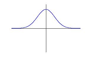
By ordering the operations a little differently, we can gain new insight into this operator. Note first that, because the Canny operator is odd symmetric, the sum of all the weights is zero. Half the weights are positive, and half are negative. We can break our summation into two parts along these lines, which now splits the signal into two sides separated by the proposed edge. We call these the "blue" (positive weight) side and the "red" (negative weight) side. The blue side is summed as before, but note that we can make the red side positive by reflecting the weights over the axis:

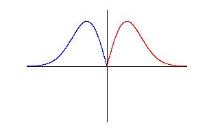Canny's operator split into two sides, with one side "flipped" so that all weights are positive

Of course, we must now subtract the red total from the blue total to get the answer, but really all we've done is to add a few negative signs.

Now let's consider what happens on one of the sides. The intensity of each pixel is multiplied by a weight. Imagine creating a histogram of intensity, where the amount that each pixel contributes is equal to the corresponding weight. What does adding these numbers mean now that our x-axis represents intensity and not location? If the total weight of a side is 1, then the answer is the center of mass of the histogram.

Two paragraphs ago we said that we had to subtract the red total from the blue total. We can actually do even better than this; if we compute the distance between the red center of mass and the blue center of mass, we get the same answer, except that now it is always non-negative. This means that we don't care whether we are moving from a dark region to a light region or vice versa.

The Perils of Smoothing

Smoothing is a weighted average of a set of pixels where the weights add up to one. The weights are often assigned using a Gaussian (normal) distribution, since Gaussians have many attractive properties. In fact, the Gaussian (actually, its derivative) forms the basis for the Canny edge detector, still the leading choice for many people because of its speed and ease of implementation, even though other operators (such as the Wang-Binford operator) have been proven to give better results.

However, a central assumption is that the image data on either side of an edge is constant with some noise. In this case, smoothing works fine. If the scale (size) of the operator increases, this can no longer hold. Also, if image regions are textured, the weighted average also has less relevance. This is especially true when color is added.

The solution, of course, is to take only local weighted averages. In other words, if a region contains blue and red and green pixels, then average the pixels of each color locally, and state the relative amounts. This is precisely the result of performing vector quantization. Smoothing is simply a special case of vector quantization where the number of colors on each side is always assumed to be one. That is the peril.

The Punch Line

It may already be clear where we are headed. If we consider a 1-D version of the compass operator, in which we allow only one cluster on each side, then the two operators are equal. The distance between the two centers of mass is exactly the answer the Earth Mover's Distance would give us.

Canny's major shortcoming, therefore, is that the center of mass of a histogram is not necessarily representative of the data in a window. When the size of the operator is kept small (as it usually is), we can assume that the image data is constant and get acceptable results. However, as we increase the scale over which we are detecting edges, the center of mass becomes more and more uninformative. (As a side note, a corollary of the work of my friend and colleague Scott Cohen says that Canny's gradient magnitude is a lower bound of the Earth Mover's Distance).

Using color only exacerbates this problem. It is visually acceptable to take a distribution of black and white pixels and choose as the center of mass a certain shade of grey. However, if we take a distribution of red and yellow and blue pixels, the color located at the center of mass (regardless of the color space used) likely does not match any of the colors in our distribution.

Two Dimensions

Canny's optimality constraints and subsequent analysis rely heavily on the fact that the signal is one-dimensional. In two dimensions, it is quite possible to have two intersecting edges or three edges meeting in a junction.

Canny does make one assumption that has been proven invalid by Sheng-Jyh Wang and Tom Binford in 1994. The gradient of a function can be computed by taking derivatives in the x- and y-directions and adding the resulting vectors together. Canny implemented this by starting with a two-dimensional Gaussian, taking a derivative in those directions, and using the results as his convolution filters. However, it is also true that a function's derivative in the direction perpendicular to the gradient (thus, along the edge) must be zero. In images, however, there is often a non-zero component along the edge (caused by shading, for instance). This means that the direction of the gradient is not always perpendicular to the edge direction, which can cause problems in the presence of planar (but not constant) surfaces, as well as at junctions and corners--precisely those parts of the image that are often the most interesting.

Wang and Binford sampled the set of possible orientations and picked the one that gave the best answer. We do the same. In addition, the minimum over all orientations (the abnormality) is also useful, both because it points out exactly where in an image Canny's assumptions are violated most severely, and also to point out places where junctions are likely to occur.

Our weighting function is the same as the "flipped" version of Canny's in one-dimension. Instead of finding another function to multiply it by in the perpendicular direction, we have chosen to rotate it out-of-plane, creating a solid of revolution (see below). This is done for computational simplicity as much as any other reason; the weights are now isotropic, whereas an anisotropic operator would require recalculation of all the weights at each orientation.

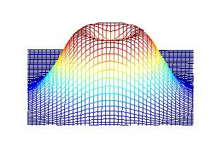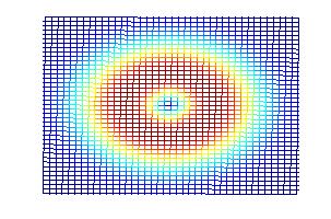Side view of compass operator	Top view of compass operator