TL;DR: Compressed sensing techniques enable efficient acquisition and recovery of sparse, high-dimensional data signals via low-dimensional projections. In our AISTATS 2019 paper, we introduce uncertainty autoencoders (UAE) where we treat the low-dimensional projections as noisy latent representations of an autoencoder and directly learn both the acquisition (i.e., encoding) and amortized recovery (i.e., decoding) procedures via a tractable variational information maximization objective. Empirically, we obtain on average a 32% improvement over competing methods on the task of statistical compressed sensing of high-dimensional data.
The broad goal of unsupervised representation learning is to learn transformations of the input data which succinctly capture the statistics of an underlying data distribution. A plethora of learning objectives and algorithms have been proposed in prior work, motivated from the perspectives of latent variable generative modeling, dimensionality reduction, and others. In this post, we will describe a new framework for unsupervised representation learning inspired from compressed sensing. We begin with a primer of statistical compressed sensing.
Statistical Compressed Sensing
Systems which can efficiently acquire and accurately recover high-dimensional signals form the basis of compressed sensing. These systems enjoy widespread use. For example, compressed sensing has been successfully applied to a wide range of applications such as designing power-efficient single-pixel cameras and accelerating scanning times of MRI for medical imaging, among many others.
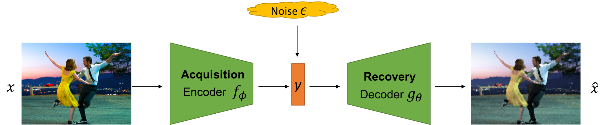
A compressed sensing pipeline consists of two components:
- Acquisition: A mapping \(f: \mathbb{R}^n \to \mathbb{R}^m\) between high-dimensional signals \(x \in \mathbb{R}^n\) to measurements \(y \in \mathbb{R}^m\)
where \(\epsilon\) is any external noise in the measurement process. The acquisition process is said to be efficient when \(m \ll n\).
- Recovery: A mapping \(g: \mathbb{R}^m \to \mathbb{R}^n\) between the measurements \(y\) to the recovered data signals \(\hat{x}\). Recovery is accurate if a normed loss e.g., \(\Vert \hat{x} - x \Vert_2\) is small.
In standard compressed sensing, the acquistion mapping \(f\) is typically linear in \(x\) (i.e., \(f(x) = Wx\) for some matrix \(W \in \mathbb{R}^{m\times n}\)). In such a case, the system is underdetermined since we have more variables (\(n\)) than constraints (\(m\)). To guarantee unique, non-trivial recovery, we assume the signals are sparse in an appropriate basis (e.g., Fourier basis for audio, wavelet basis for images). Thereafter, acquisition via certain classes of random matrices and recovery by solving a LASSO optimization method guarantees unique recovery with high probability using only a few measurements (roughly logarithmic in the data dimensionality).
In this work, we consider the setting of statistical compressed sensing where we have access to a dataset \(\mathcal{D}\) of training data signals \(x\). We assume that every signal \(x \stackrel{i.i.d.}{\sim} q_{\textrm{data}}\) for some unknown data distribution \(q_{\textrm{data}}\). One way to think about acquisition and recovery in this setting is to consider a game between an agent and nature.
At training time:
- Nature shows the agent a finite dataset \(\mathcal{D}\) of high-dimensional signals.
- Agent learns the acquistion and recovery mappings \(f\) and \(g\) by optimizing a suitable objective.
At test time:
- Nature shows the agent the compressed measurements \(y = f(x) + \epsilon\) for one or more test signals \(x \stackrel{i.i.d.}{\sim} q_{\textrm{data}}\).
- Agent recovers the signal as \(\hat{x} = g(y)\) and incurs an \(\ell_2\)-norm loss \(\Vert \hat{x} - x \Vert_2\).
To play this game, the agent’s task is to choose the acquisition and recovery mappings \(f\) and \(g\) such that the test loss is minimized.
Uncertainty Autoencoders
In practice, there are two sources of uncertainty in recovering the signal \(x\) from the measurements \(y\) alone, even if the agent is allowed to pick an acquisition mapping \(f\). One is due to the stochastic measurement noise \(\epsilon\). Second, the acquisition mapping \(f\) is typically parameterized with a family of finite-precision restricted mappings \(\Phi\) (e.g., linear mappings as in standard compressed sensing or more generally neural networks). Given that the dimensionality of the measurements \(y\) is smaller than that of the signal \(x\), such restrictions would prohibit learning a bijective mapping even in the absence of noise.
For the illustrative case where the mapping \(f\) is linear, we established that exact recovery is not possible. Then what are some other ways to efficiently acquire data? In the figure below, we consider a toy setting where the true data distribution is an equally-weighted mixture of two 2D Gaussians stretched along orthogonal directions. We sample 100 points (black) from this mixture and consider two methods to reduce the dimensionality of these points to one dimension.
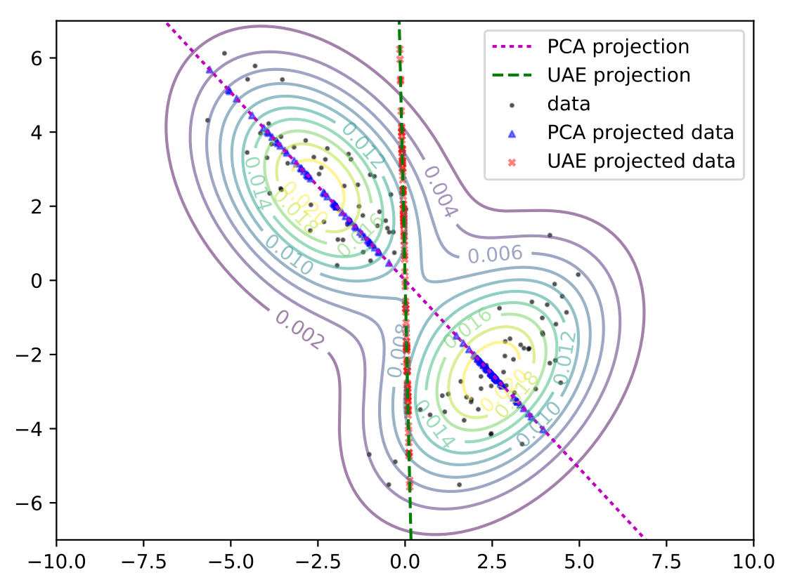
One option is to project the data along directions that account most for the variability in the data using principal component analysis (PCA). For the 2D example above, this is shown via the blue points on the magenta line. This line captures a large fraction of the variance in the data but collapses data sampled from the bottom right Gaussian into a narrow region. When multiple datapoints are collapsed into overlapping, densely clustered regions in the low-dimensional space, disambiguating the association between the low-dimensional projections and the original datapoints is difficult during recovery.
Alternatively, we can consider the projections (red points) on the green axis. These projections are more spread out and suggest that recovery is easier, even if doing so increases the total variance in the projected space compared to PCA. Next, we present the UAE framework which learns precisely the aforementioned low-dimensional projections that make recovery more accurate1.
Probabilistically, the joint distribution of the signal \(x\) and measurements \(y\) is given as \(q(x, y) = q_{\textrm{data}} (x) q_\phi (y \vert x)\). E.g., if we model the noise as centered isotropic Gaussian, the likelihood \(q_\phi(y \vert x)\) can be expressed as \(q_\phi(y \vert x) = \mathcal{N}(y \mid f_\phi(x), \sigma^2)\). To learn the parameters \(\phi\in \Phi\) that best facilitate recovery in the presence of uncertainty, consider the following objective
\[\phi^\ast = \arg\max_{\phi \in \phi} E_{q_\phi(x, y)}[\log q_\phi(x \vert y)] : = \mathcal{L}(\phi).\]The above objective maximizes the log-posterior probability of recovering \(x\) from the measurements \(y\), consistent with the agent’s goal at test time as mentioned above.
Variational Information Maximization
Alternatively, one can interpret the above as maximizing the mutual information between the signals \(x\) and the measurements \(y\). To see the connection, note that the data entropy \(H(x)\) is a constant and does not affect the optima. Hence, we can rewrite the objective as
\[\phi^\ast = \arg\max_{\phi \in \Phi} E_{q_\phi(x, y)}[\log q_\phi(x \vert y)] + H(X) = -H_\phi(X \vert Y) + H (X) = I_\phi(X;Y).\]Evaluating (and optimizing) the mutual information is unfortunately non-trivial and intractable in the current setting. To get around this difficulty while also permitting fast recovery, we propose to use an amortized variant of the variational lower bound on mutual information due to 2.
In particular, we consider a parameterized, variational approximation \(p_\theta (x \vert y )\) to the true posterior \(q_\phi( x \vert y)\). Here, \(\theta \in \Theta\) denote the variational parameters. Substituting the variational distribution gives us the following lower bound to the original objective
\[\mathcal{L}(\phi) \geq E_{q_\phi(x, y)}[\log p_\theta(x \vert y)] := \mathcal{L}(\phi, \theta).\]The above expression defines the learning objective for uncertainty autoencoders, where acquisition can be seen as encoding the data signals and recovery corresponds to decoding the signals from the measurements.
Example
In practice, the expectation in the UAE objective is evaluated via Monte Carlo: the data signal \(x\) is sampled from the training dataset \(\mathcal{D}\), and the measurements \(y\) are sampled from an assumed noise model that permits reparameterization (e.g., isotropic Gaussian). Depending on the accuracy metric of interest for recovery, we can make a distributional assumption on the amortized variational distribution \(p_\theta(x \vert y)\) (e.g., Gaussian with fixed variance for \(\ell_2\), Laplacian for \(\ell_1\)) and map the measurements \(y\) to the sufficient statistics of \(p_\theta(x \vert y)\) via the recovery mapping \(g_\theta\).
As an illustration, consider an isotropic Gaussian noise model \(q_\phi(y \vert x)\) with known scalar variance \(\sigma^2\). If we also let the variational distribution \(p_\theta(x \vert y)\) be an isotropic Gaussian with fixed scalar variance, we obtain the following objective maximized by an uncertainty autoencoder (UAE)
\[\mathcal{L}(\phi, \theta) \approx - c \sum_{x \in \mathcal{D}} \sum_{y \sim \mathcal{N}(y \mid f_\phi(x), \sigma^2)} \Vert x - g_\theta(y)\Vert_2\]for some positive normalization constant \(c\) that is independent of \(\phi\) and \(\theta\).
Comparison with commonly used autoencoders
Even beyond statistical compressive sensing, UAEs present an alternate framework for unsupervised representation learning where the compressed measurements can be interpreted as the latent representations. Below, we discuss how UAEs computationally differ and relate to commonly used autoencoders.
- Standard autoencoders (AE): In the absence of any noise in the latent space, the UAE learning objective reduces to that of an AE.
- Denoising autoencoders (DAE)3: A DAE adds noise in the observed space (i.e., to the data signals), whereas a UAE models the uncertainty in the latent space.
- Variational autoencoders (VAE)4: A VAE regularizes the latent space to follow a prior distribution. There is no explicit prior in a UAE, and consequently no KL divergence regularization of the distribution over the latent space5. This avoids pitfalls of representation learning with VAEs where the latent representations are ignored in the presence of powerful decoders6.
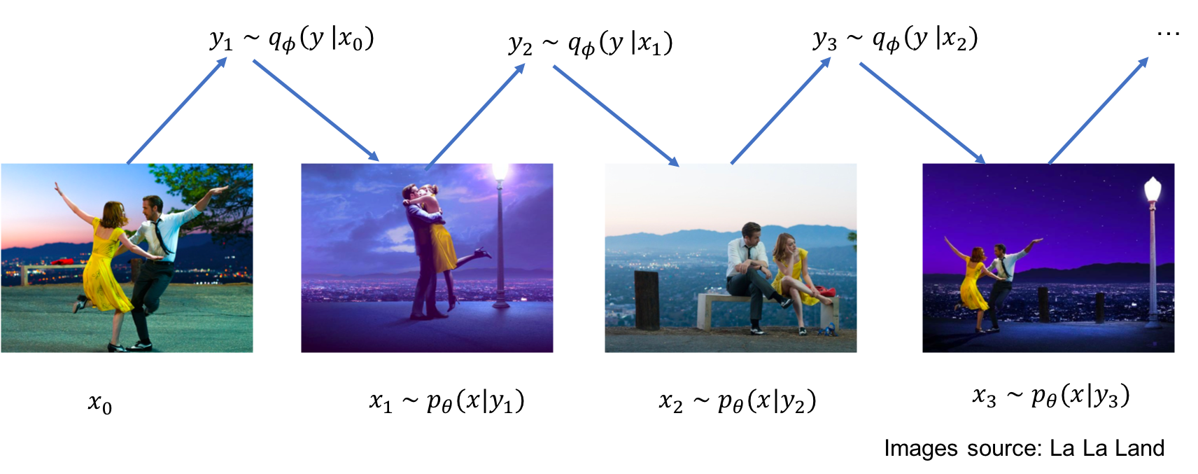
Does a UAE permit out-of-sample generalization, like a DAE or a VAE? Yes! Under suitable assumptions, we show that a UAE learns an implicit generative model of the data signal distribution and can be used to define a Markov chain Monte Carlo sampler. See Theorem 1 and Corollary 1 in the paper for more details.
Overview of experimental results
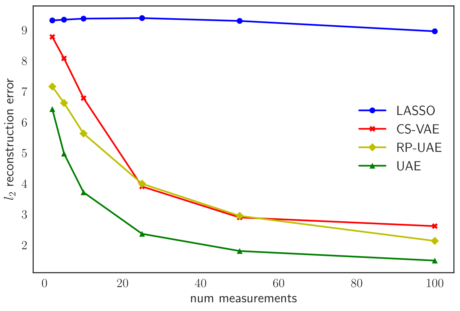
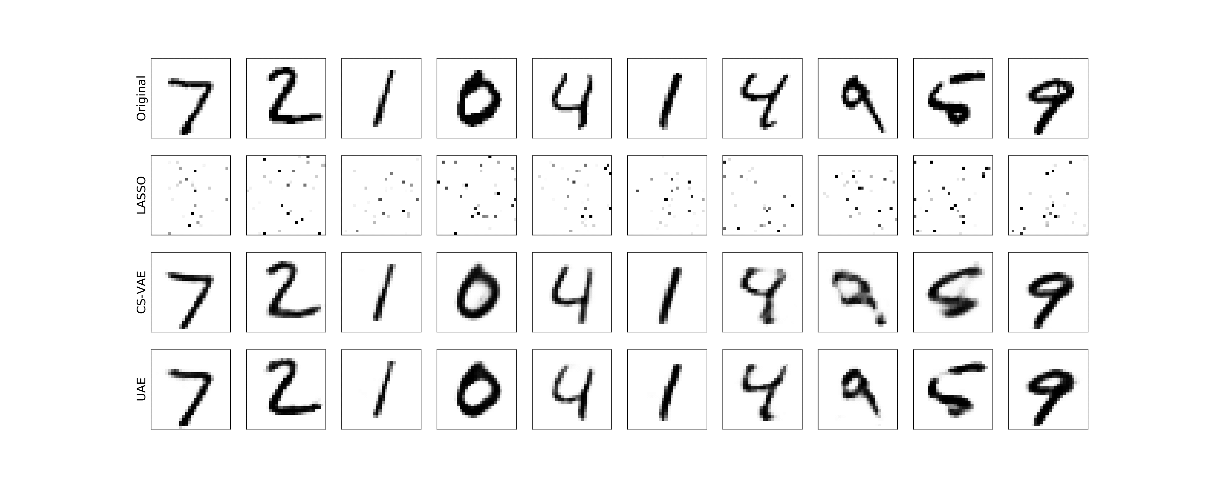
We present some experimental results on statistical compressive sensing of image datasets below for varying numbers of measurements \(m\) and random Gaussian noise. We compare against two baselines:
- LASSO in an appropriate sparsity-inducing basis
- CS-VAE/DCGAN7, a recently proposed compressed sensing method that searches the latent space of pretrained generative models such as VAEs and GANs for the latent vectors that minimize the recovery loss.
MNIST
CelebA
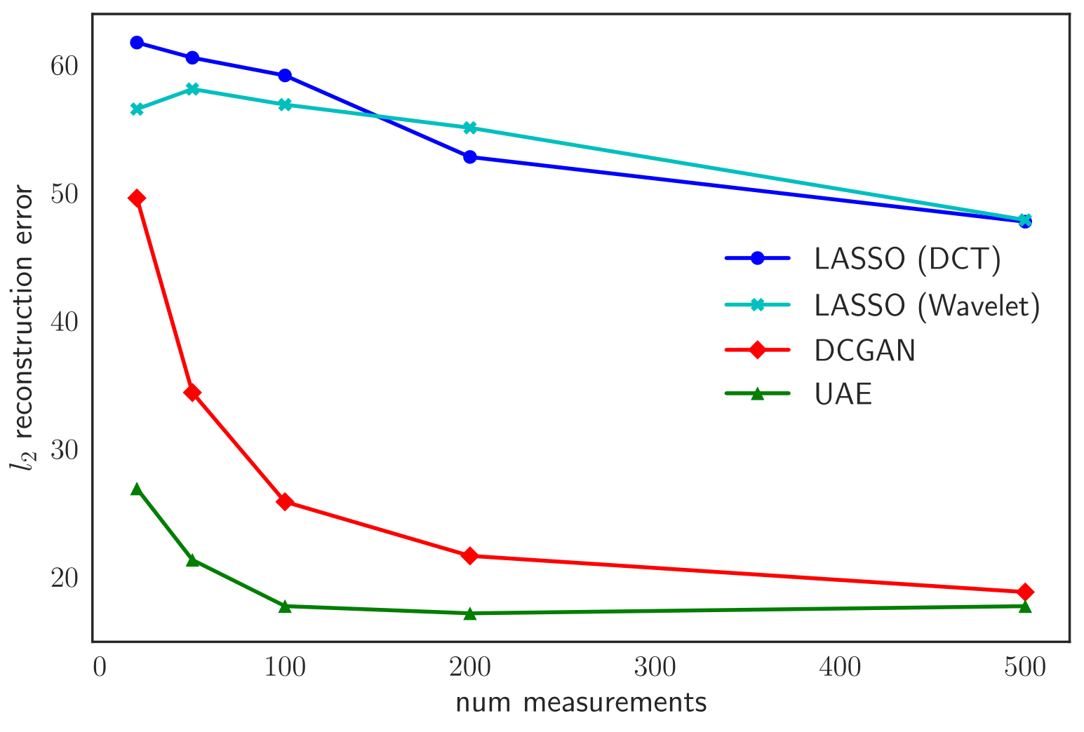
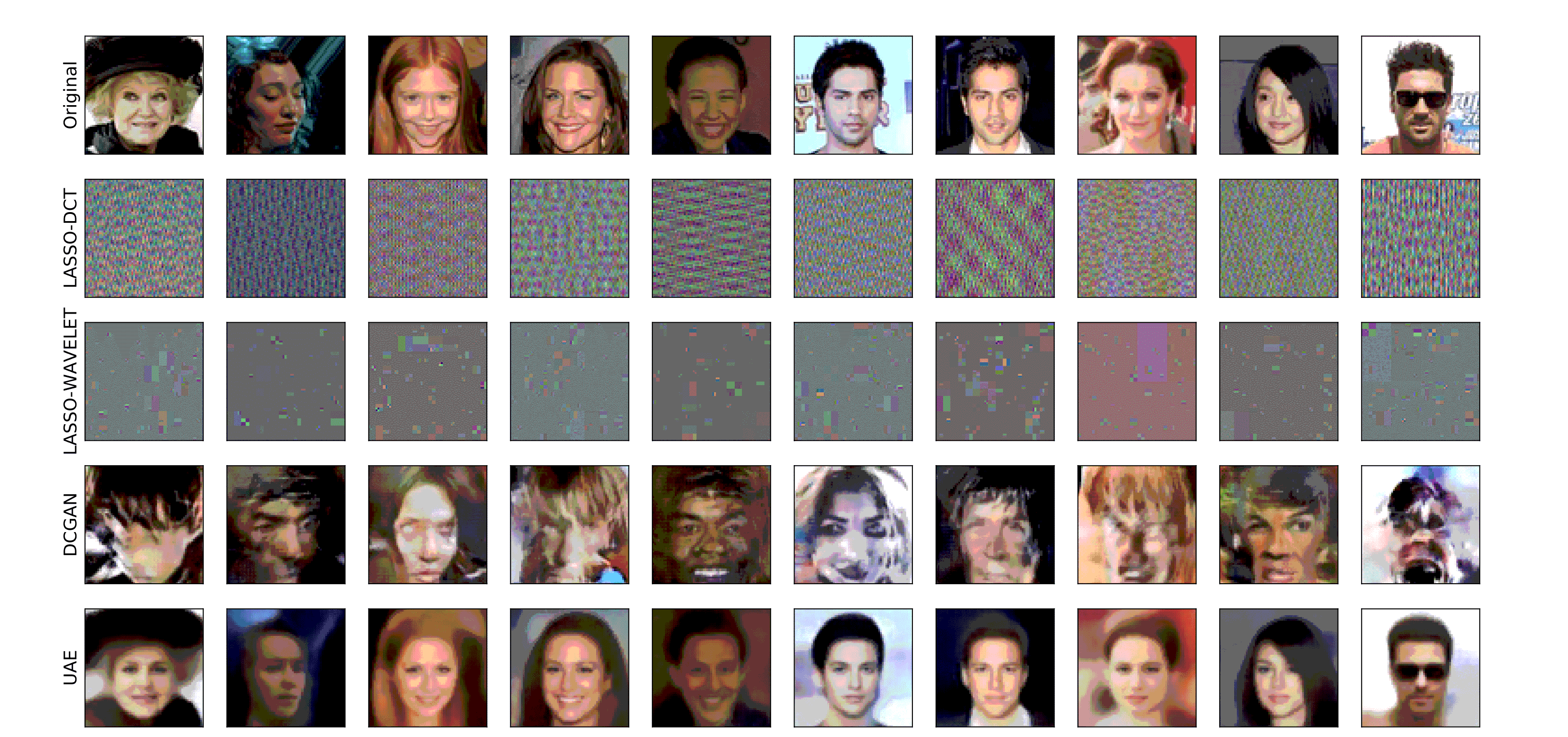
On average, we observe a 32% improvement across all datasets and measurements. For results on more datasets and tasks involving applications of UAE to transfer learning and supervised learning, check out our paper below!
Uncertainty Autoencoders: Learning Compressed Representations via Variational Information Maximization. Aditya Grover, Stefano Ermon. AISTATS, 2019. paper, code
This post was shared earlier on the Ermon group blog.
-
We show in Theorem 2 in the paper that in the case of a Gaussian noise model, PCA is a special case of the information maximizing objective for a linear encoder and optimal (potentially non-linear) decoder under suitable assumptions. ↩
-
Agakov, David Barber Felix. “The IM Algorithm: a Variational Approach to Information Maximization.” In Advances in Neural Information Processing Systems, 2004. ↩
-
Vincent, Pascal, Hugo Larochelle, Yoshua Bengio, and Pierre-Antoine Manzagol. “Extracting and Composing Robust Features with Denoising Autoencoders.” In ICML, 2008. ↩
-
Kingma, Diederik P, and Max Welling. “Auto-Encoding Variational Bayes.” In ICLR, 2014. ↩
-
While not discussed in the original paper, the UAE objective can be seen as a special case of the \(\beta\)-VAE objective for \(\beta=0\). Higgins, Irina, Loic Matthey, Arka Pal, Christopher Burgess, Xavier Glorot, Matthew Botvinick, Shakir Mohamed, and Alexander Lerchner. 2016. “Beta-Vae: Learning Basic Visual Concepts with a Constrained Variational Framework.” In ICLR, 2017. ↩
-
Chen, Xi, Diederik P Kingma, Tim Salimans, Yan Duan, Prafulla Dhariwal, John Schulman, Ilya Sutskever, and Pieter Abbeel. “Variational Lossy Autoencoder.” In ICLR, 2017. ↩
-
Bora, Ashish, Ajil Jalal, Eric Price, and Alexandros G Dimakis. 2017. “Compressed Sensing Using Generative Models.” In ICML, 2017. ↩