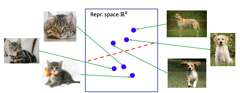
Labels for large-scale datasets are expensive to curate, so leveraging abundant unlabeled data before fine-tuning them on the smaller, labeled, data sets is an important and promising direction for pre-training machine learning models. One popular and successful approach for developing pre-trained models is contrastive learning, (He et al., 2019, Chen et al., 2020). Contrastive learning is a powerful class of self-supervised visual representation learning methods that learn feature extractors by (1) minimizing the distance between the representations of positive pairs, or samples that are similar in some sense, and (2) maximizing the distance between representations of negative pairs, or samples that are different in some sense. Contrastive learning can be applied to unlabeled images by having positive pairs contain augmentations of the same image and negative pairs contain augmentations of different images.

In this blog post, we will propose a theoretical framework for understanding the success of this contrastive learning approach. Our theory motivates a novel contrastive loss with theoretical guarantees for downstream linear-probe performance. Our experiments suggest that representations learned by minimizing this objective achieve comparable performance to state-of-the-art methods.
Augmentation graph for self-supervised learning
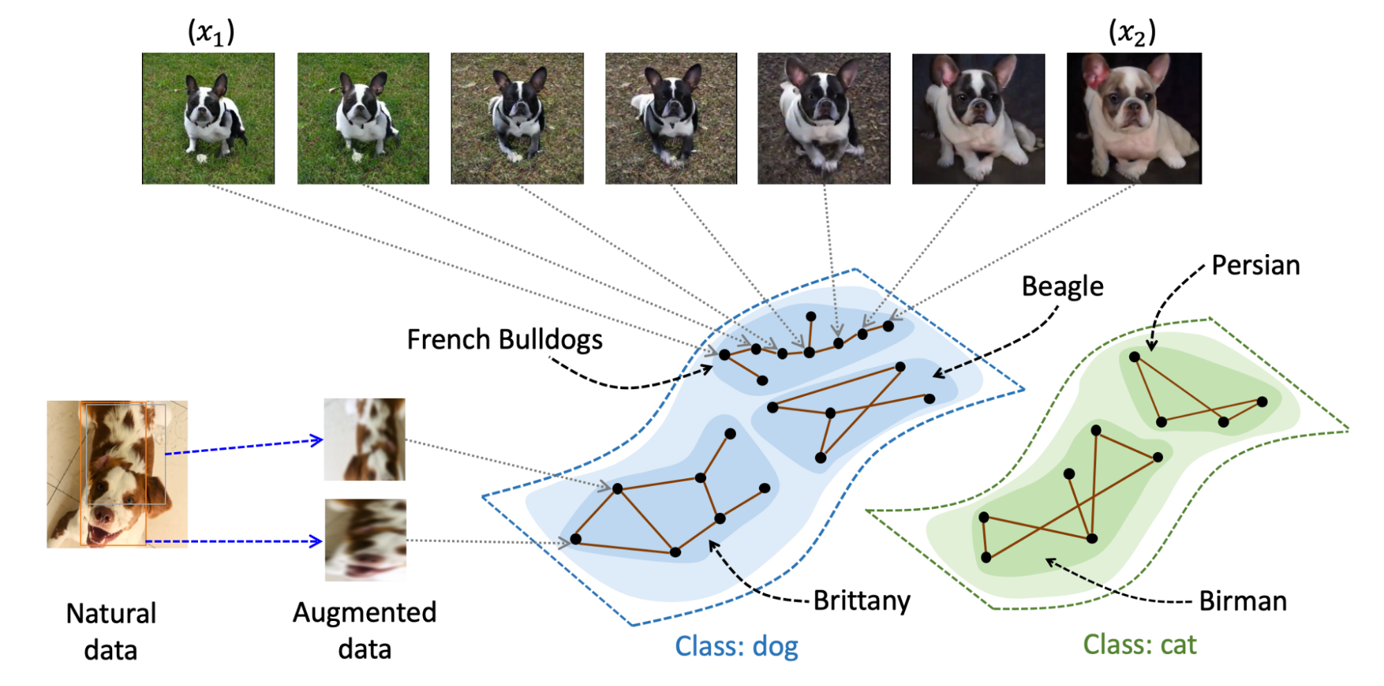
The key idea behind our work is the idea of a population augmentation graph, which also appeared in our previous blog post where we analyzed self-training. As a reminder, this graph is built such that the nodes represent all possible augmentations of all data points in the population distribution and the edges connect nodes that are derived from the same natural image. Further, the edges are weighted to be the probability that the two augmented images are augmentations of the same underlying image, given the set of augmentation functions being used. Some augmentation methods, like cropping, produce images that could only come from the same underlying image. However, others, such as Gaussian blurring, technically connect all images to each other, albeit mostly with very small probabilities. Because there are a potentially infinite number of augmentations, this graph is more of a theoretical idea we will use to describe our idea rather than an actual graph that we construct. The figure below gives a visualization of the graph, where augmented images of French bulldogs are connected in the graph.

We have two simple intuitions about the graph that suggests it contains information generally useful for a pre-trained computer vision model. First, very few high-probability edges exist between any two images, especially if they have different semantic content. For instance, consider two pictures of the same dogs in different poses. Even though the semantic content is the same, there is almost zero chance that one could produce one image from the other using augmentation methods like Gaussian blur. This probability is reduced further when considering two images that don’t even share the same objects, such as one image of a dog outside and another image of a cruise ship in the ocean. Rather, the only high-probability connections are augmented images with similar objects in similar orientations or poses. Second, images with similar content (e.g, dog images of the same breed) can be connected to each other via a path of interpolating images. The figure above visualizes this intuition, where \(x_1\) and \(x_2\) are two augmented images of French bulldogs that aren’t obtained from the same natural image (hence no high-probability edge between them). However, since the augmentation graph is a theoretical construct that is defined on the population data which contains all possible dog images, there must exist a path of interpolating French bulldog images (as shown in Figure 1) where every consecutive two images are directly connected by a reasonably high-probability edge. As a result, this sequence forms a path connecting \(x_1\) and \(x_2\).
Graph partitioning via spectral decomposition
Consider an ideal world where we can partition the augmentation graph into multiple disconnected subgraphs. From the intuition above, each subgraph contains images that can be easily interpolated into each other, and so likely depicts the same underlying concept or objects in its images. This motivates us to design self-supervised algorithms that can map nodes within the same subgraph to similar representations. Assume we have access to the population data distribution and hence the whole augmentation graph. A successful algorithm for graph partitioning is spectral clustering (Shi & Malik 2000, Ng et al. 2002), which uses spectral graph theory tools to discover the connected components in a graph. We’ll describe spectral clustering in more detail here, and then interpret contrastive learning as an effective, parametric way to implement spectral clustering on the large augmentation graph. Let X denote the vertex set of the graph, and for the ease of exposition assume \( |X| = N\). (\(N\) can also be infinite or exponential.) Let \(A\in \mathbb{R}^{N\times N}\) be the adjacency matrix which contains edge weights \(w_{xx’}\) as its entries. For every node \(x\), let \(w_x=\sum_{x’\in X} w_{xx’}\) be the sum of weights of edges connected to x (which can be thought of as the degree of the vertex \(x\)). We call the matrix \(L=I-\text{diag}(w_x^{-1/2})\cdot A \cdot \text{diag}(w_x^{-1/2})\) the Laplacian matrix of the graph. Spectral clustering begins with eigendecomposition of the Laplacian matrix. Let \(u_1, u_2, \cdots, u_{k}\) be the \(N\)-dimensional eigenvectors that correspond to the smallest \(k\) eigenvalues. If we write these vectors as columns of a matrix \(F \in \mathbb{R}^{N\times k}\), every row (denoted as \(v_1, v_2, \cdots, v_N \in \mathbb{R}^{k}\)) would correspond to a single node in the graph. We can then obtain a \(k\)-way partition of the graph by running \(k\)-means on these \(N\) vectors.

It’s worth noting that we cannot directly run spectral clustering on the population augmentation graph, since its eigendecomposition step requires knowing the entire graph (i.e., all the data in the population), whereas in reality we only have a sampled dataset. However, the intuition behind spectral clustering is still valuable: the smallest eigenvectors of the Laplacian matrix should provide pretty good representations of the data.
Contrastive learning as spectral clustering
We can use these intuitions about spectral clustering to design a contrastive learning algorithm. Specifically, because we don’t have access to the true population augmentation graph, we instead define \(f_\theta\) which is a neural network that takes in an example and outputs the eigenvector representation of the example. Put another way, our goal is to compute the matrix \(F\) that contains the eigenvectors as columns, and use its rows as the representations. We aim to learn \(f_\theta\) such that \(f_\theta(x)\) is the row of matrix \(F\) corresponding to example \(x\). Given the high expressivity of neural nets, we assume that such a \(\theta\) exists.

It turns out that this feature can be learned by minimizing the following “matrix factorization loss”:
\[\min_{F_\theta}L(F_\theta) \triangleq \left\| (I-L) - F_\theta F_\theta^\top \right\|_F^2 =\sum_{i, j} \left(\frac{w_{x_ix_j}}{\sqrt{w_{x_i}}\sqrt{w_{x_j}}} - f_\theta(x_i)^\top f_\theta(x_j)\right)^2\]where \(F_\theta\in\mathbb{R}^{N\times k}\) is the matrix containing \(f_\theta(x_i)\) as its \(i\)-th row. According to the Eckart–Young–Mirsky theorem, any minimizer of this loss contains the largest eigenvectors of \(I-L\) (hence the smallest eigenvectors of \(L\)) as its columns(up to scaling). As a result, at the minimizer, \(f_\theta\) recovers the smallest eigenvectors. We expand the above loss, and arrive at a formula that (somewhat surprisingly) resembles a contrastive loss:
\[\begin{aligned} \min_{\theta} L(f_\theta) &= \text{const} -2\sum_{i, j}\frac{w_{x_ix_j}}{\sqrt{w_{x_i}}\sqrt{w_{x_j}}}f_\theta(x_i)^\top f_\theta(x_j) + \sum_{i, j}\left(f_\theta(x_i)^\top f_\theta(x_j)\right)^2 \\ &= \text{const} -2\mathbb{E}_{x,x^+}\frac{f_\theta(x)^\top}{\sqrt{w_x}}\frac{f_\theta(x^+)}{\sqrt{w_{x^+}}} + \mathbb{E}_{x,x'}\left(\frac{f_\theta(x)^\top}{\sqrt{w_x}}\frac{f_\theta(x')}{\sqrt{w_{x'}}}\right)^2 \end{aligned}\]where \((x, x^+)\) is a random positive pair and \((x, x’)\) is a random negative pair. In the second line, we are using the fact that \(w_{x_ix_j}\) and \(w_{x_i}w_{x_j}\) are the probability densities of \((x_i, x_j)\) being a positive and negative pair, respectively, to replace the sums by expectations. Ignoring the constant term and the scalings \(\sqrt{w_x}\) (which do not influence linear separability of the learned representations), we get the following contrastive loss objective \(\min_{\theta} L_{\text{scl}}(f_\theta) = -2\mathbb{E}_{x,x^+} \left[f_\theta(x)^\top f_\theta(x^+)\right] + \mathbb{E}_{x,x'}\left[\left(f_\theta(x)^\top f_\theta(x')\right)^2\right]\) which we call spectral contrastive loss. The minimizer of this objective would correspond to the smallest eigenvectors of the Laplacian matrix with some data-wise positive scaling. In summary, the above analysis shows that, when minimizing a special variant of contrastive loss (i.e., spectral contrastive loss), the learned features correspond to the eigenvectors of the Laplacian matrix of the population augmentation graph.

Empirically, features learned by training spectral contrastive loss can match strong baselines such as SimCLR and SimSiam. The above table shows the linear probe accuracy with 100-epoch pre-training on ImageNet. More discussions about the empirical performance of this loss can be found in the experiments section of our paper.
Why does this method produce good representations?
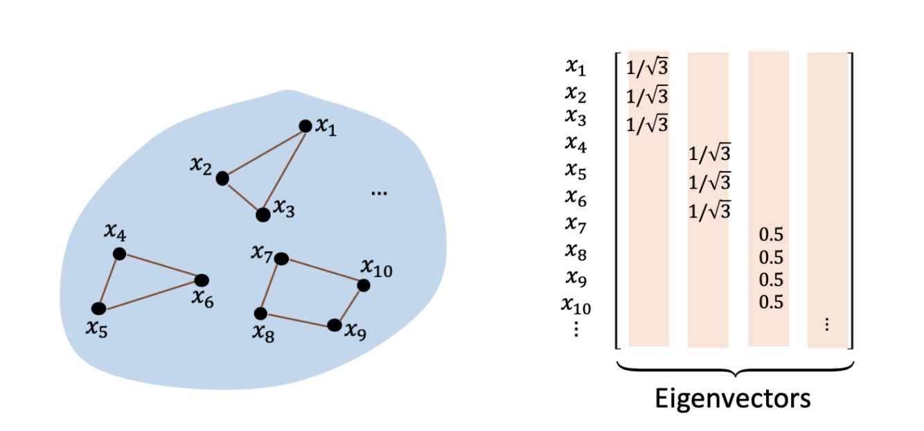
We now turn to the question we began with: why are the representations learned by contrastive loss useful for downstream computer vision tasks? We study the downstream accuracy of the representation with the “linear probe” protocol (Chen et al. 2020), where an additional linear model is trained on the representation to predict the labels for a downstream classification task. As discussed above, the representations learned by the spectral contrastive loss are the rows (with data-wise positive scaling) of a matrix where the columns are the smallest eigenvectors of the Laplacian matrix. Since the scaling doesn’t change the linear prediction, it suffices to consider the rows of the eigenvector matrix as representations. The usefulness of this representation in classification tasks can be demonstrated by the following didactic example: consider a augmentation graph \(G\) with three completely disconnected components that correspond to three classes, and the downstream task is to classify one component (e.g., set \(\{x_1, x_2, x_3\}\) versus the rest).

The figure above shows the smallest eigenvectors of the Laplacian, where the blank entries are 0. It’s easy to see that here rows of the eigenvector matrix exactly correspond to indicators of different components in the graph, and hence the representations of nodes from different connected subgraphs are clearly linearly separable. For instance, if we use the sign of \(f(x)^\top b\) as the predictor where vector \(b\in\mathbb{R}^{k}\) is set to be \(e_1\), we can perfectly classify whether a node belongs to set \(\{x_1, x_2, x_3\}\) or not. The same intuition holds in a broader setting where the graph isn’t regular, the components aren’t necessarily disconnected, and the downstream task has more than two classes. In summary, the contrastive learned representation can linearly predict any set of nearly disconnected components with high accuracy, which is captured by the following theorem: Theorem (informal): Assume the population augmentation graph contains \(k\) approximately disconnected components, where each component corresponds to a downstream class. Let the feature map \(f: X\rightarrow \mathbb{R}^k\) be the minimizer of the population spectral contrastive loss. Then, there exists a linear head on top of \(f\) that achieves small downstream classification error. The formal version of this theorem can be found in our paper.
Conclusion
Our theory suggests that self-supervised learning can learn quite powerful and diverse features that are suitable for a large set of downstream tasks. To see this, consider a situation where there are a large number of disconnected subgraphs in the augmentation graph, the downstream task can be an arbitrary way of grouping these subgraphs into a small number of classes (each class can correspond to many subgraphs, .e.g., the “dog” class may contain many subgraphs corresponding to different breeds of dogs). Due to the abundance of unlabeled data in practice, generalization in the traditional sense (i.e., studying population loss vs. empirical loss) is no longer the main challenge to understanding self-supervised learning. Instead, a good understanding of the population pretraining loss and its connection with the downstream tasks becomes essential. As a result, proper modeling of the pretraining data becomes key to the theoretical analysis. We hope that our theoretical framework, which characterizes properties of the data via the augmentation graph, can facilitate a better understanding of unsupervised algorithms in deep learning and can inspire new practical loss functions and algorithms. This blog post was based on our NeurIPS 2021 paper Provable Guarantees for Self-Supervised Deep Learning with Spectral Contrastive Loss.