Deep models require a lot of training examples, but labeled data is difficult to obtain. This motivates an important line of research on leveraging unlabeled data, which is often more readily available. For example, large quantities of unlabeled image data can be obtained by crawling the web, whereas labeled datasets such as ImageNet require expensive labeling procedures. In recent empirical developments, models trained with unlabeled data have begun to approach fully-supervised performance (e.g., Chen et al., 2020, Sohn et al., 2020).
This series of blog posts will discuss our theoretical work which seeks to analyze recent empirical methods which use unlabeled data. In this first post, we’ll analyze self-training, which is a very impactful algorithmic paradigm for semi-supervised learning and domain adaptation. In Part 2, we will use related theoretical ideas to analyze self-supervised contrastive learning algorithms, which have been very effective for unsupervised representation learning.
Background: self-training
We will first provide a basic overview of self-training algorithms, which are the main focus of this blog post. The core idea is to use some pre-existing classifier \(F_{pl}\) (referred to as the “pseudo-labeler”) to make predictions (referred to as “pseudo-labels”) on a large unlabeled dataset, and then retrain a new model with the pseudo-labels. For example, in semi-supervised learning, the pseudo-labeler is obtained from training on a small labeled dataset, and is then used to predict pseudo-labels on a larger unlabeled dataset. A new classifier \(F\) is then retrained from scratch to fit the pseudo-labels, using additional regularization. In practice, \(F\) will often be more accurate than the original pseudo-labeler \(F_{pl}\) (Lee 2013). The self-training procedure is depicted below.
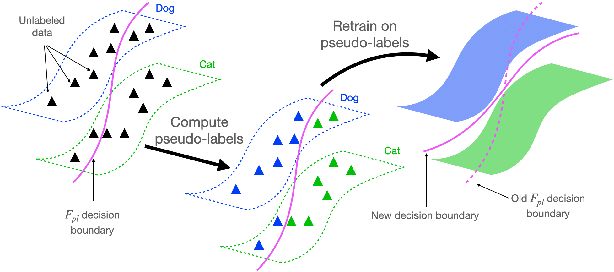
It is quite surprising that self-training can work so well in practice, given that we retrain on our own predictions, i.e. the pseudo-labels, but not the true labels. In the rest of this blogpost, we’ll share our theoretical analysis explaining why this is the case, showing that retraining in self-training provably improves accuracy compared to the original pseudo-labeler.
Our theoretical analysis focuses on pseudo-label-based self-training, but there are also other variants. For example, entropy minimization, which essentially trains on changing pseudo-labels produced by \(F\), rather than fixed pseudo-labels from \(F_{pl}\), can also be interpreted as self-training. Related analysis techniques apply to these algorithms (Cai et al. ‘21).
The importance of regularization for self-training
Before discussing core parts of our theory, we’ll first set up the analysis by demonstrating that regularization during the retraining phase is necessary for self-training to work well.
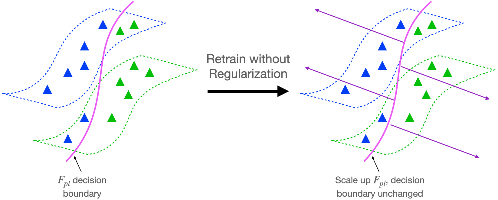
Let’s consider the retraining step of the self-training algorithm described above. Suppose we minimize the cross-entropy loss to fit the pseudo-labels, as is the case for deep networks. It’s possible to drive the unregularized cross-entropy loss to 0 by scaling up the predictions of \(F_{pl}\) to infinity. As depicted in Figure 2 below, this means that the retraining step won’t achieve any improvement over \(F_{pl}\) because the decision boundary will not change. This suggests that regularization might be necessary to have in our analysis if self-training is to lead to provable improvements over the pseudo-labeler.
Empirically, one technique which leads to substantial improvements after the retraining step is to encourage the classifier to have consistent predictions on neighboring pairs of examples. We refer to such methods as forms of input consistency regularization. In the literature, there are various ways to define “neighboring pairs”, for example, examples close in \(\ell_2\) distance (Miyato et al., 2017, Shu et al., 2018), or examples which are different strong data augmentations of the same image (Xie et al., 2019, Berthelot et al., 2019, Xie et al., 2019, Sohn et al., 2020). Strong data augmentation, which applies stronger alterations to the input image than traditionally used in supervised learning, is also very useful for self-supervised contrastive learning, which we will analyze in the follow-up blog post. Our theoretical analysis considers a regularizer which is inspired by empirical work on input consistency regularization.
Key formulations for theoretical analysis
From the discussion above, it’s clear that in order to understand why self-training helps, we need a principled way to think about the regularizer for self-training. Input consistency regularization is effective in practice, but how do we abstract it so that the analysis is tractable? Furthermore, what properties of the data does the input consistency regularizer leverage in order to be effective? In the next section we’ll introduce the augmentation graph, a key concept that allows us to cleanly resolve both challenges. Building upon the augmentation graph, subsequent sections will formally introduce the regularizer and assumptions on the data.
Augmentation graph on the population data
We introduce the augmentation graph on the population data, a key concept which allows us to formalize the input consistency regularizer and motivates natural assumptions on the data distribution.
Intuitively, the augmentation graph is a graph with data points as vertices with the property that semantically similar data points will be connected by sequences of edges. We will consider the bipartite graph \(G’\) displayed in Figure 3 below, whose vertex set consists of all natural images \(X\) as well as the set \(\tilde{X}\) of augmented versions of images in \(X\). The graph contains an edge (in pink) between \(x \in X\) and \(\tilde{x} \in \tilde{X}\) if \(\tilde{x}\) is obtained by applying data augmentation to \(x\).
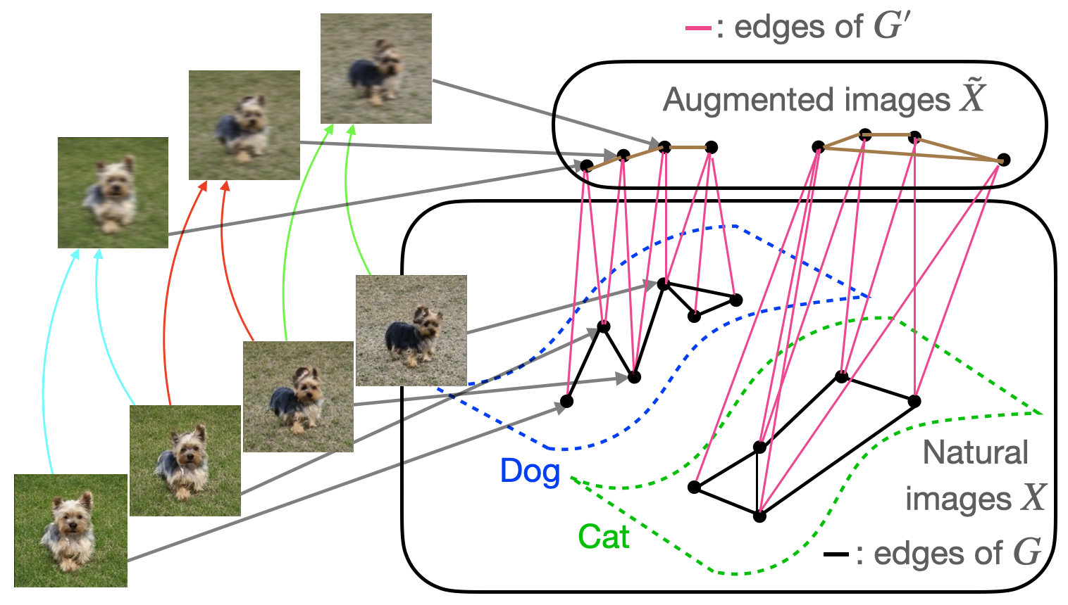
The analysis will be slightly simpler if we work with the graph \(G\) obtained by collapsing \(G’\) onto the vertex set \(X\). Edges of \(G\) are shown in black and connect vertices \(x_1, x_2 \in X\) which share a common neighbor in \(G’\). Natural images \(x_1, x_2 \in X\) are neighbors in \(G\) if and only if they share a common neighbor in \(G’\). In our next post on self-supervised contrastive learning algorithms, we will also consider the graph obtained by collapsing \(G’\) onto \(\tilde{X}\), whose edges are shown in brown in the figure above.
For simplicity, we only consider unweighted graphs and focus on data augmentations which blur the image with small \(\ell_2\)-bounded noise, although the augmentation graph can be constructed based on arbitrary types of data augmentation. The figure above shows examples of neighboring images in \(G\), with paired colored arrows pointing to their common augmentations in \(\tilde{X}\). Note that by following edges in \(G\), it is possible to traverse a path between two rather different images, even though neighboring images in \(G\) are very similar and must have small \(\ell_2\) distance from each other. An important point to stress is that \(G\) is a graph on the population data, not just the training set – this distinction is crucial for the type of assumptions we will make about \(G\).
Formalizing the regularizer
Now that we’ve defined the augmentation graph, let’s see how this concept helps us formulate our analysis. First, the augmentation graph motivates the following natural abstraction for the input consistency regularizer:
\[R(F, x) = 1(F \text{ predicts the same class on all examples in neighborhood } N(x)) \tag{1}\]In this definition, the neighborhood \(N(x)\) is the set of all \(x’\) such that \(x\) and \(x’\) are connected by an edge in the augmentation graph. The final population self-training objective which we will analyze is a sum of the regularizer and loss in fitting the pseudo-label and is closely related to empirically successful objectives such as in (Xie et al., 2019, Sohn et al., 2020).
\[E_x[1(F(x) \ne G_{pl}(x))] + \lambda E_x[R(F, x)] \tag{2}\]Assumptions on the data
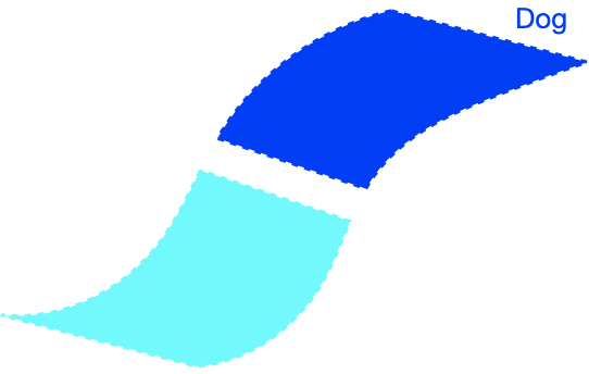
We will now perform a thought experiment to see why the regularizer is useful, and in doing so motivate two key assumptions for our analysis. Let’s consider an idealized case where the classifier has perfect input consistency, i.e., \(R(F, x) = 0\) for all \(x\). If the data satisfies an appropriate structure, enforcing perfect input consistency can be very advantageous, as visualized below.
The figure above demonstrates that if the dog class is connected in \(G\), enforcing perfect input consistency will ensure that the classifier makes the same prediction on all dogs. This is because the perfect input consistency ensures that the same label propagates through all neighborhoods of dog examples, eventually covering the entire class. This is beneficial for avoiding overfitting to incorrectly pseudolabeled examples.
There were two implicit properties of the data distribution in Figure 4 which ensured that the perfect input consistency was beneficial: 1) The dog class was connected in \(G\), and 2) The dog and cat classes were far apart. Figure 5 depicts failure cases where these conditions don’t hold, so the perfect input consistency does not help. The left shows that if the dog class is not connected in \(G\), perfect input consistency may not guarantee that the classifier predicts the same label throughout the class. The right shows that if the dog and cat classes are too close together, perfect input consistency would imply that the classifier cannot distinguish between the two classes.
Our main assumptions, described below, are natural formalizations of the conditions above.
Assumption 1 (Expansion within classes): The augmentation graph has good connectivity within classes. Formally, for any subset \(S\) of images within a ground-truth class, \(P(N(S)) > cP(S)\) for some \(c > 1\).
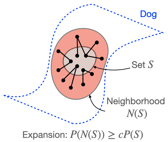
The figure above illustrates Assumption 1. In Assumption 1, \(N(S)\) refers to the neighborhood of \(S\), which contains \(S\) and the union of neighborhoods of examples in \(S\). We refer to Assumption 1 as the “expansion” assumption because it requires that the neighborhood of \(S\) must expand by a constant factor \(c\) in probability relative to \(S\) itself. We refer to the coefficient \(c\) as the expansion coefficient. Intuitively, larger \(c\) implies better connectivity because it means each set has a larger neighborhood. Related notions of expansion have been studied in the past in settings such as spectral graph theory [2,3], sampling and mixing time [4], combinatorial optimization [5], and even semi-supervised learning in a different co-training setting [1].
Assumption 2 (Separation between classes): There is separation between classes: the graph \(G\) does contains a very limited number of edges between different classes.
In the paper, we provide examples of distributions satisfying expansion and separation, and we believe that they are realistic characterizations of real data. One key point to reiterate is that these assumptions and the graph \(G\) are defined for population data. Indeed, it is not realistic to have properties such as expansion hold for the training set. If we were to attempt to build the graph \(G\) on only training examples, it would be completely disconnected because the probability of drawing two i.i.d. samples which happen to be neighbors (defined over \(\ell_2\) distance) is exponentially small in the input dimension.
Main theoretical results
We now show that a model satisfying low self-training loss (2) will have good classification accuracy. Our main result is as follows:
Theorem 1 (informal): There exists a choice of input consistency regularization strength \(\lambda\) such that if the pseudo-labeler satisfies a baseline level of accuracy, i.e., \(\text{Error}(G_{pl}) < 1/3\), the minimizer \(\hat{F}\) of the population objective (2) will satisfy:
\[\text{Error}(\hat{F}) \le \frac{2}{c - 1} \text{Error}(G_{pl})\]In other words, assuming expansion and separation, self training provably leads to a more accurate classifier than the original pseudo-labeler! One of the main advantages of Theorem 1 is that it does not depend on the parameterization of \(F\), and, in particular, holds when \(F\) is a deep network. Furthermore, in the domain adaptation setting, we do not require any assumptions about the relationship between the source and target domain, as long as the pseudo-labeler hits the baseline accuracy level. Prior analyses of self-training were restricted to linear models (e.g., Kumar et al. 2020, Chen et al. 2020), or domain adaptation settings where the domain shift is assumed to be very small (Kumar et al. 2020).
An interesting property of the bound is that it improves as the coefficient \(c\) in the expansion assumption gets larger. Recall that \(c\) essentially serves as a quantifier for how connected the augmentation graph is within each class, and larger \(c\) indicates more connectivity. Intuitively, connectivity can improve the bound by strengthening the impact of the input consistency regularizer.
One way to improve the graph connectivity is to use stronger data augmentations. In fact, this approach has worked very well empirically: algorithms like FixMatch and Noisy Student achieve state-of-the-art semi-supervised learning performance by using data augmentation which alters the images much more strongly than in standard supervised learning. Theorem 1 suggests an explanation for why strong data augmentation is so helpful: it leads to a larger \(c\) and a smaller bound. However, one does need to be careful to not increase augmentation strength by too much – using too strong data augmentation could make it so that our Assumption 2 that ground truth classes are separated would no longer hold.
The proof of Theorem 1 relies on the intuition conveyed in the previous subsection. Recall that the goal is to show that retraining on pseudo-labels can lead to a classifier which corrects some of the mistakes in the pseudo-labels. The reason why the classifier can ignore some incorrect pseudo-labels is that the input consistency regularization term in (2) encourages the classifier to predict the same label on neighboring examples. Thus, we can hope that the correctly pseudo-labeled examples will propagate their labels to incorrectly pseudo-labeled neighbors, leading to a denoising effect on these neighbors. We can make this intuition rigorous by leveraging the expansion assumption (Assumption 1).
The main result of Theorem 1 and our assumptions were phrased for population data, but it’s not too hard to transform Theorem 1 into accuracy guarantees for optimizing (2) on a finite training set. The key observation is that even if we only optimize the training version of (2), because of generalization, the population loss will also be small, which is actually sufficient for achieving the accuracy guarantees of Theorem 1.
Conclusion
In this blog post, we discussed why self-training on unlabeled data provably improves accuracy. We built an augmentation graph on the data such that nearby examples are connected with an edge. We assumed that two examples in the same class can be connected via a sequence of edges in the graph. Under this assumption, we showed that self-training with regularization improves upon the accuracy of the pseudo-labeler by enforcing each connected subgraph to have the same label. One limitation is that the analysis only works when the classes are fine-grained, so that each class forms its own connected component in the augmentation graph. However, we can imagine scenarios where one large class is a union of smaller, sparsely connected subclasses. In these cases, our assumptions may not hold. Our follow-up blog post on contrastive learning will show how to deal with this case.
This blog post was based on the paper Theoretical Analysis of Self-Training with Deep Networks on Unlabeled Data.
Additional references
- Balcan MF, Blum A, Yang K. Co-training and expansion: Towards bridging theory and practice. Advances in neural information processing systems; 2005.
- Cheeger J. A lower bound for the smallest eigenvalue of the Laplacian. Problems in analysis; 2015.
- Chung FR, Graham FC. Spectral graph theory. American Mathematical Soc.; 1997.
- Kannan R, Lovász L, Simonovits M. Isoperimetric problems for convex bodies and a localization lemma. Discrete & Computational Geometry; 1995.
- Mohar B, Poljak S. Eigenvalues and the max-cut problem. Czechoslovak Mathematical Journal; 1990.