Introduction
Discriminatory behavior towards certain groups by machine learning (ML) models is especially concerning in critical applications such as hiring. This blog post explains one source of discrimination: the reliance of ML models on different groups’ data distributions. We will show that when ML models use noisy features (which are pervasive in the real world, e.g., exam scores), they’re incentivized to devalue a good candidate from a lower-performing group. This blog post is based on:
Fereshte Khani and Percy Liang, “Feature Noise Induces Loss Discrepancy Across Groups.” International Conference on Machine Learning. PMLR, 2020
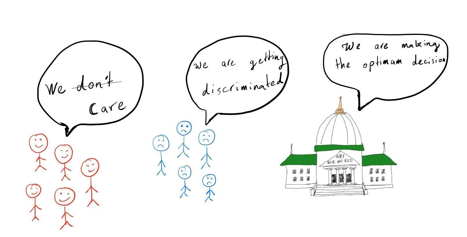
The findings are illustrated by reviewing the hiring process in the fictitious city of Ney, where recently a group of people has accused the government of discrimination.
Hiring people in Ney
The government of Ney wants to hire qualified people. Each person in Ney has a skill level that is normally distributed with a mean \(\mu\) and a standard deviation of \(\sigma_\text{skill}\). A person is qualified if their skill level is greater than 0 and non-qualified otherwise. The government wants to hire qualified people (all people with skills greater than 0). For example, Alice with skill level 2, is qualified, but Bob with the skill level of -1 is not qualified.
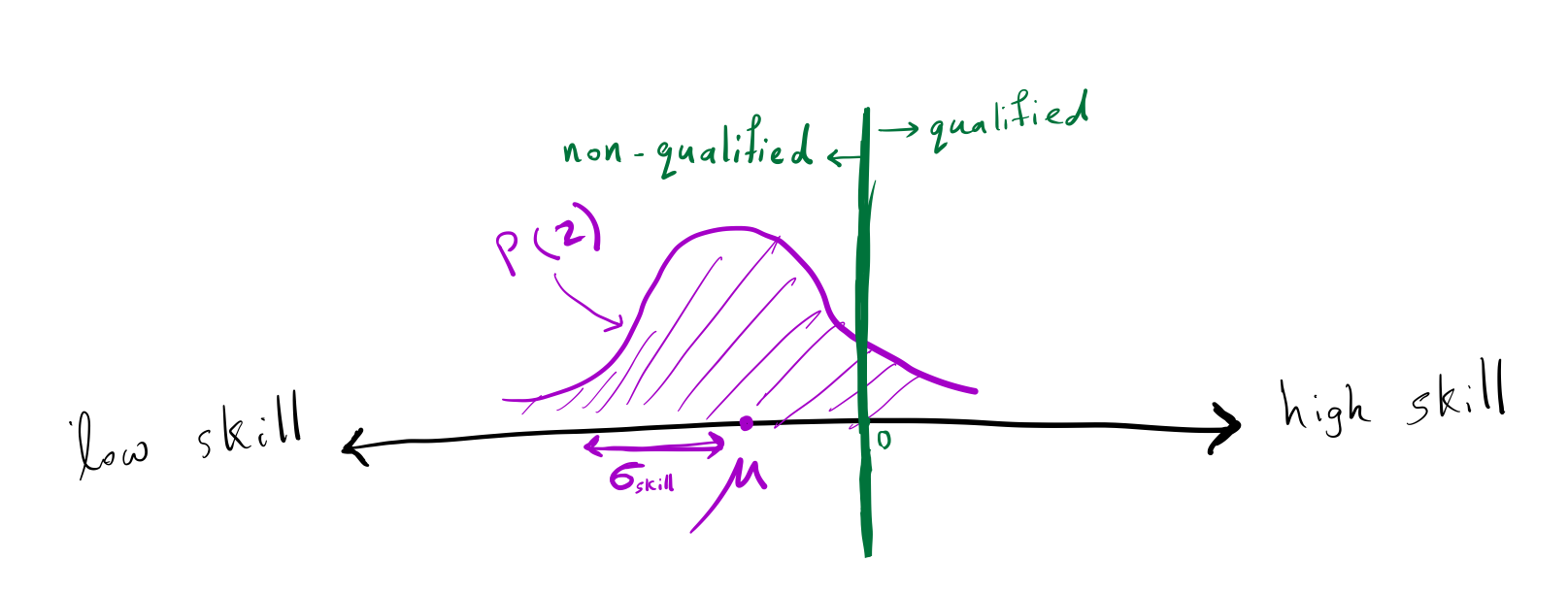 The skills level of the people in Ney is normally distributed with a mean of \(\mu\) and a standard deviation of \(\sigma_\text{skill}\).
To assess people’s skills, the government created an exam. The exam score is a noisy indicator of the applicant’s skill since it cannot capture the true skill of a person (e.g., the same applicant would score differently on different versions of SAT). In the city of Ney, exam noise is nice and simple: If an individual has skill \(z\), then their score is distributed as \(\mathcal{N} (z, \sigma_\text{noise}^2)\), where \(\sigma_\text{noise}^2\) indicates the variance of noise on the exam.
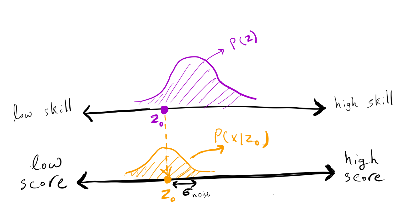 The exam score of an individual with a skill of \(z\) is a random variable normally distributed with a mean of \(z\) and a standard deviation of \(\sigma_\text{noise}\).
The government wants to choose a threshold \(\tau\), and hire all people whose exam scores are greater than \(\tau\). There are two kinds of errors that the government can make:
- Not hiring a qualified person (\(z > 0 \land x \le \tau\))
- Hiring a non-qualified person (\(z \le 0 \land x > \tau\))
For simplicity, let’s assume the government cares about these two types of errors equally and wants to minimize the overall error, i.e., the number of non-qualified hired people plus the number of qualified non-hired people.
\[\begin{align} \text{Error} = \mathbb{E}\left[[z>0] \neq [x > \tau]\right]\\ \end{align}\]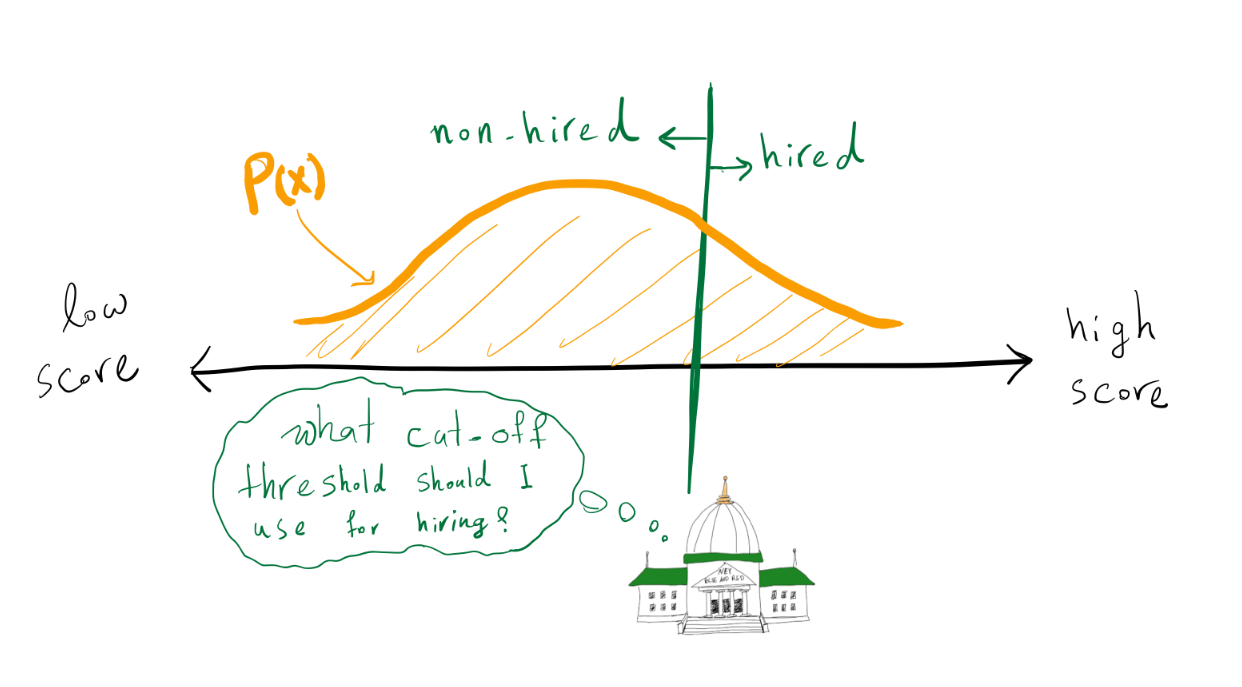 The government’s goal is to find a cut-off threshold such that it minimizes the error.
Given all exam scores and knowledge of the skill distribution of the people, what cut-off threshold should the government use to minimize the error (the above equation)? Is it a good strategy for the government to simply use 0 as the threshold and hire all individuals with scores greater than zero?
Let’s consider an example where the skill distribution is \(\mathcal{N}(-1,1)\), and the exam noise has a standard deviation of \(\sigma_\text{noise}=1\). The following lines of code plot the average error for various thresholds for this example. As illustrated, 0 is not the best threshold to use. In fact, in this example, a threshold of \(\tau=1\) leads to minimum error.
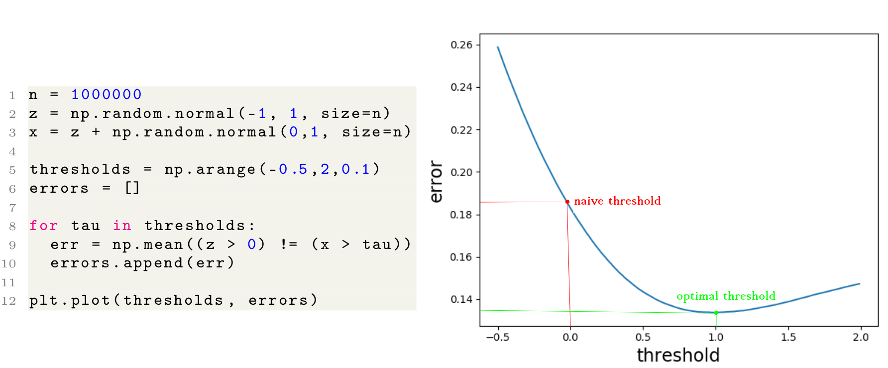 A simple example with \(\mu=-1\) and \(\sigma_\text{skill}=\sigma_\text{noise}=1\). As shown on the right, accepting individuals with a score higher than \(0\) does not result in the minimum error.
The government wants to minimize the number of hired people with negative skill levels + the number of non-hired people with positive skill levels. Hiring all people with positive exam scores (a noisy indicator of the skill) is not optimal.
If 0 is not always the optimal threshold, then what is the optimal threshold for minimizing error for different values of \(\mu, \sigma_\text{skill}\) and \(\sigma_\text{noise}\)? Generally, given a person’s exam score (\(x\)) and the skill level distribution (\(\mathbb{P}(z)\)), what can we infer about their real skill (\(z\))? Here is where Bayesian inference comes in.
Bayesian inference
Let’s see what we can infer about a person’s skill given their exam score and knowing the skill level distribution \(\mathbb{P} (z)\) (known as the prior distribution since it shows the prior over a person’s skill). Using Bayes rule, we can calculate \(\mathbb{P} (z|x)\) (known as the posterior distribution since it shows the distribution over a person’s skill after observing their score).
Let’s first consider two extreme cases:
- If the exam is completely precise (i.e., \(\sigma_\text{noise}=0\)), then the exam score is the exact indicator of a person’s skill (irrespective of the prior distribution).
- If the exam is pure noise (i.e., \(\sigma_\text{noise} \rightarrow \infty\)), then the exam score is meaningless, and the best estimate for a person’s skill is the average skill \(\mu\) (irrespective of the exam score).
Intuitively, when the noise variance has a value between \(0\) and \(\infty\), the best estimate of a person’s skill is a number between their exam score (\(x\)) and the average skill (\(\mu\)). The figure below shows the standard formulation of the posterior distribution \(\mathbb{P} (z \mid x)\) after observing an exam score (\(x_0\)). For more details on how to derive this formula, see this.
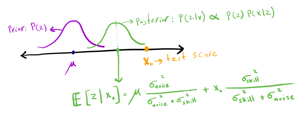 Posterior distribution of a person’s skill after observing their exam score (\(x_0\)).
Based on this formula (and as hypothesized), depending on the amount of noise, \(\mathbb{E} [z\mid x]\) is a number between \(x\) and \(\mu\).
An applicant’s expected skill level is between their exam score and the average skill among Ney people. If the exam is noisier, it is closer to the average skill; if the exam is more precise, it is closer to the exam score.
Optimal threshold
Now that we have exactly characterized the posterior distribution (\(\mathbb{P} (z \mid x)\)), the government can find the optimal threshold. For any exam score \(x\), if the government hires people with score \(x\), it incurs \(\mathbb{P}(z \le 0 \mid x) \) error (probability of hiring non-qualified people). On the other hand, if it does not hire people with score \(x\), it incurs \(\mathbb{P}(z > 0 \mid x)\) error (probability of non-hiring qualified people). Thus, in order to minimize the error, the government should hire a person iff \(\mathbb{P} (z > 0 \mid x) > \mathbb{P}(z \le 0 \mid x)\). Since the posterior distribution is a normal distribution, the government must hire an applicant iff \(\mathbb{E}[z \mid x] > 0\).
Using the formulation in the previous section, we have:
\[\begin{align}\mu \frac{\sigma_\text{noise}^2}{\sigma_\text{noise}^2 + \sigma_\text{skill}^2} + x \frac{\sigma_\text{skill}^2}{\sigma_\text{skill}^2 + \sigma_\text{noise}^2} > 0 \iff x > -\mu \frac{\sigma_\text{noise}^2}{\sigma_\text{skill}^2} \end{align}\]Therefore, the optimal threshold is:
\[\bbox[5px, border: 2px solid grey]{ \text{optimal threshold} = -\mu\frac{\sigma_\text{noise}^2}{\sigma_\text{skill}^2} }\]In our running example with average skill \(\mu=-1\) and \(\sigma_\text{skill} = \sigma_\text{noise}=1\), the optimal threshold is 1. The figure below shows how the optimal threshold varies according to \(\mu\) and \(\sigma_\text{noise}\). As \(\sigma_\text{noise}\) increases or \(\mu\) decreases, the optimal threshold moves farther away from \(0\).
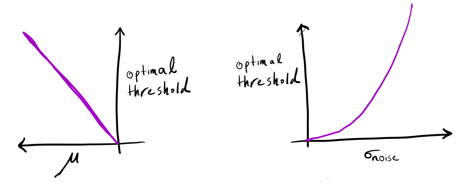 (left) The optimal threshold increases as the average of the prior distribution decreases (with a fixed exam noise \(\sigma_\text{noise} > 0\)). (right) The optimal threshold increases if the exam noise increases (with a fixed average skill \(\mu < 0\)). Note that, if exam scores are not noisy or the average skill is zero, then the optimal threshold is zero.
As exams become more noisy or the average skill becomes more negative, the optimal threshold moves further away from 0.
What does machine learning have to do with all of this?
So far, we precisely identified the optimal cut-off threshold given the exact knowledge of \(\mu, \sigma_\text{skill}\), and \(\sigma_\text{noise}\). But how can the government find the optimal threshold using observational data? This is where machine learning (ML) comes into the picture. Let’s imagine very favorable conditions. Let’s assume everyone (an infinite number of them!) takes the exam, the government hires all of them and observes their true skills. Further, assume the modeling assumption is perfectly correct (i.e., both the true prior distribution and conditional distribution are normal). What would happen if the government trains a model with an infinite number of \((x,z)\) pairs?
 The government has collected lots of data and now wants to use ML models to predict the best threshold that minimizes the error.
Before delving into this, we would like to note that in real-world scenarios, we do not have infinite data (finite data issues); the government does not hire everyone (selection bias issues), and the true skill is not perfectly observable (target noise/biases issues). Furthermore, the modeling assumptions are often incorrect (model misspecification issues). Each of these issues may affect the model adversely; however, in this blog post our goal is to analyze the model decisions when none of these issues exist. In the next section, we will show that discrimination occurs even under these ideal conditions.
Under these very favorable conditions and the right loss function, machine learning algorithms can perfectly predict \(\mathbb{E} [z \mid x]\) from \(x\); therefore, can find the optimal threshold that minimizes the error. The following few lines of Python code show how linear regression and logistic regression fit the data. In this example, we set \(\mu = -1, \sigma_\text{skill}=\sigma_\text{noise}=1\), and as shown in the figure on the right, the cut-off threshold predicted by the model is one, which matches the optimal threshold as we observed previously.
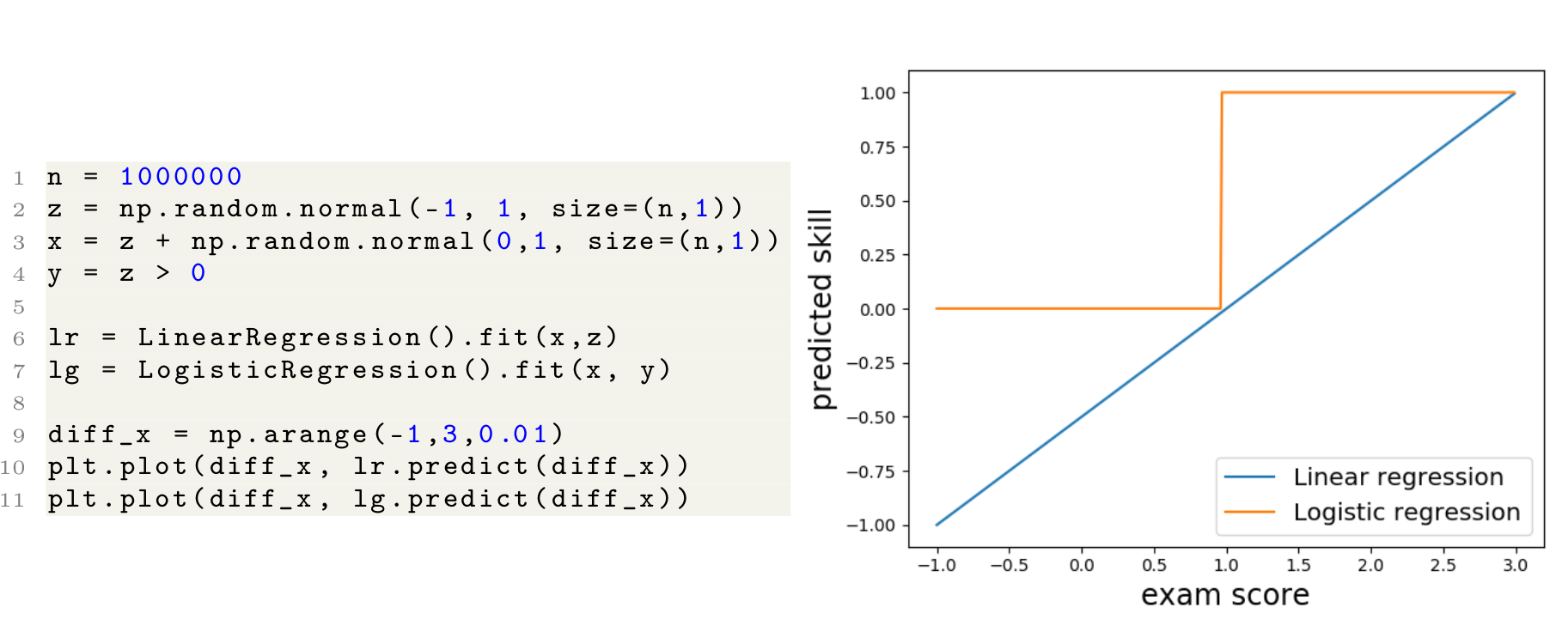 A simple example along with the predicted cut-off
threshold for linear and logistic regression. The predicted cut-off
threshold results in the minimum error, as previously discussed.
A simple example along with the predicted cut-off
threshold for linear and logistic regression. The predicted cut-off
threshold results in the minimum error, as previously discussed.
Under very favorable conditions, machine learning models find the optimal threshold, which is a function of average skill, exam noise, and skill variance among people.
Optimal thresholds for different groups
So far, we have shown how to calculate the optimal threshold and illustrated that ML models also recover this threshold. Let’s now analyze the optimal threshold when different groups exist in the population. There are two kinds of people in the city of Ney: blue and red. The blue people’s skills are normally distributed centered on \(\mu_\text{blue}\), and the red people’s skills are normally distributed centered on \(\mu_\text{red}\). The standard deviation for both groups is \(\sigma_\text{skill}\). There can be various reasons for disparities between groups, for example historically blue people might not have been allowed to attend school.
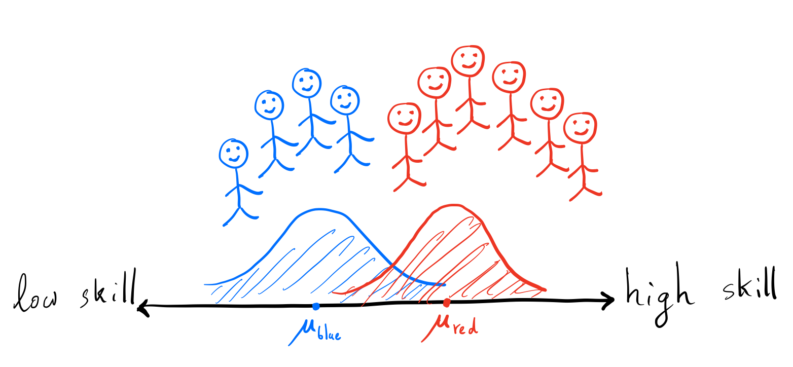 In Ney, people are divided into two groups: blue and red. The blue people have a lower average skill level than the red people.
First of all, let’s see what happens if the exam is completely precise. As previously discussed in this case, the optimal threshold to use is 0 for both groups independent of their distribution. Thus, both groups are held to the same standard, and the error for the government is 0.
If there is no noise in the exam, then zero is the optimal threshold for both groups and leads to zero error.
Now let’s analyze the case where the exam is noisy ( \(\sigma_\text{noise} > 0\)). As discussed in the prior sections, the optimal threshold depends on the average of the prior distribution, thus the optimal threshold differs between blue and red groups. Therefore, if the government knows the demographic information, then it’s a better strategy for the government to classify different groups separately (in order to minimize the error). In particular, the government can calculate the optimal threshold for blue and red people using Bayesian inference.
\[\begin{align} \text{Red Threshold} = -\mu_\text{red} \frac{\sigma_\text{noise}^2}{\sigma_\text{skill}^2} \quad \quad \text{Blue Threshold} = -\mu_\text{blue}\frac{\sigma_\text{noise}^2}{\sigma_\text{skill}^2} \end{align}\]People in a group that has lower average skills need to pass a higher bar for hiring! Not only do blue people need to overcome other associated effects of being in a group with lower average skills, they also need to pass a higher bar to get hired.
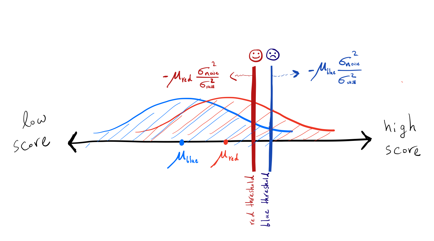 The cut-off threshold for hiring is higher for blue people in comparison to the red people.
As stated, the government uses a higher threshold for people in a group with a lower average skill! Consider two individuals with the same skill level but from different groups. The blue person is less likely to get hired by the government than the red person. Surprisingly, blue people who are already in a group with a lower average skill (which probably affects their confidence and society’s view of them) need to also pass a higher bar to get hired!
Finally, note that the gap between thresholds for the different groups grows as the noise increases.
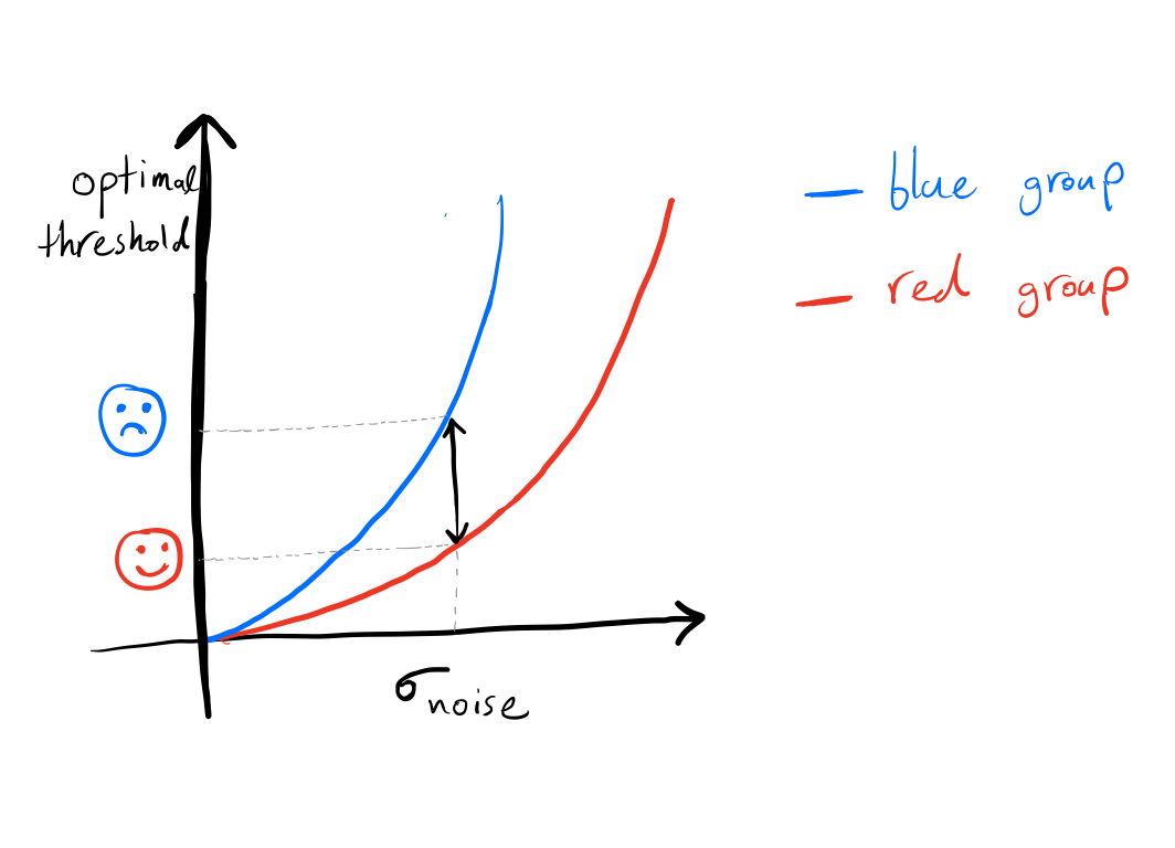 As the exam noise increases, the gap between the optimal thresholds among different groups widens. Blue people need to get a better score than red people on the exam to get hired.
A blue person has a lower chance of getting hired in comparison with a red person with the same skill.
Conclusion
We examined the discriminatory effect of relying on noisy features. When ML models use noisy features, they’re naturally incentivized to devalue a good score when the candidate in question comes from an overall lower-performing group. Note that noisy features are prevalent in any real-world application (here, we assumed that noise is the same among all individuals, but it’s usually worse for disadvantaged groups). Ideally, we would like to improve the features to better reflect a candidate’s skill/potential or make the features more closely approximate the job requirements. If that’s not possible, it’s important to be conscious that the “optimal decision” is to discriminate, and we should adjust our process (e.g., hiring) in acknowledgment that group membership can shade an individual’s evaluation.
Frequently asked questions
Can we just remove the group membership information, so the model treats individuals from both groups similarly?
Unlike this example where group membership is a removable feature, real-world datasets are more complex. Usually, datasets contain many features such that the group membership can be predicted from them (recall that ML models benefit from predicting group membership since it lowers error). Thus, it is not obvious how to remove group membership in these datasets. See [1,2,3] for some efforts on removing group information.
Why should we treat these two groups similarly when their distributions are inherently different? Utilizing group membership information reduces error overall and for both groups!
Fairness in machine learning usually studies the impact of ML algorithms on groups according to protected attributes such as sex, sexual orientation, race, etc. Usually, there has been some discrimination towards these groups throughout history, which leads to huge disparities among their distributions. For example, women (because of their sex) were not allowed to go to universities. Thus, these disparities are not inherent and could (and probably should!) change over time. For instance, see women in the labor force [4].
Another reason to avoid relying on disparities among protected groups in models is feedback loops. Feedback loops might exacerbate distributional disparities among protected groups over time. (e.g., few women get accepted → the self-doubt between women increases → women perform worse in the exam → fewer women get accepted and so on). For instance, see [5] and [6].
Finally, note that although the government objective may be to minimize the error by weighting the costs of hiring non-qualified and non-hiring qualified candidates similarly, it is not clear whether the group objectives should be the same. For example, a group might be worse off as a result of the government not hiring its qualified members than if the government had hired its non-qualified members (for example, in settings where the lack of minority role models in higher-level positions leads to a lower perceived sense of belonging in other members of a group). Thus, using group membership to minimize the error is not necessarily the most beneficial outcome for a group; and depending on the context we might need to minimize other objectives.
What about other notions of fairness in machine learning?
In this blog post, we studied the ML model’s prediction for two similar individuals (here same z) but from different groups (blue vs. red). This is referred to as the counterfactual notion of fairness. There is another common notion of fairness known as the statistical notion of fairness, which looks at the groups as a whole and compares their incurred error (it is also common to compare the error incurred by qualified members of different groups known as the equal opportunity [7]). Statistical and counterfactual notions of fairness are independent of each other, and satisfying one does not guarantee satisfying the other. Another consequence of feature noise is causing a trade-off between these two notions of fairness, which is beyond this blog post’s scope. See our paper [8] for critiques regarding these two notions and the effect of feature noise on statistical notions of fairness.
Acknowledgement
I would like to thank Percy Liang, Megha Srivastava, Frieda Rong, and Rishi Bommasani, Yeganeh Alimohammadi, and Michelle Lee for their useful comments.