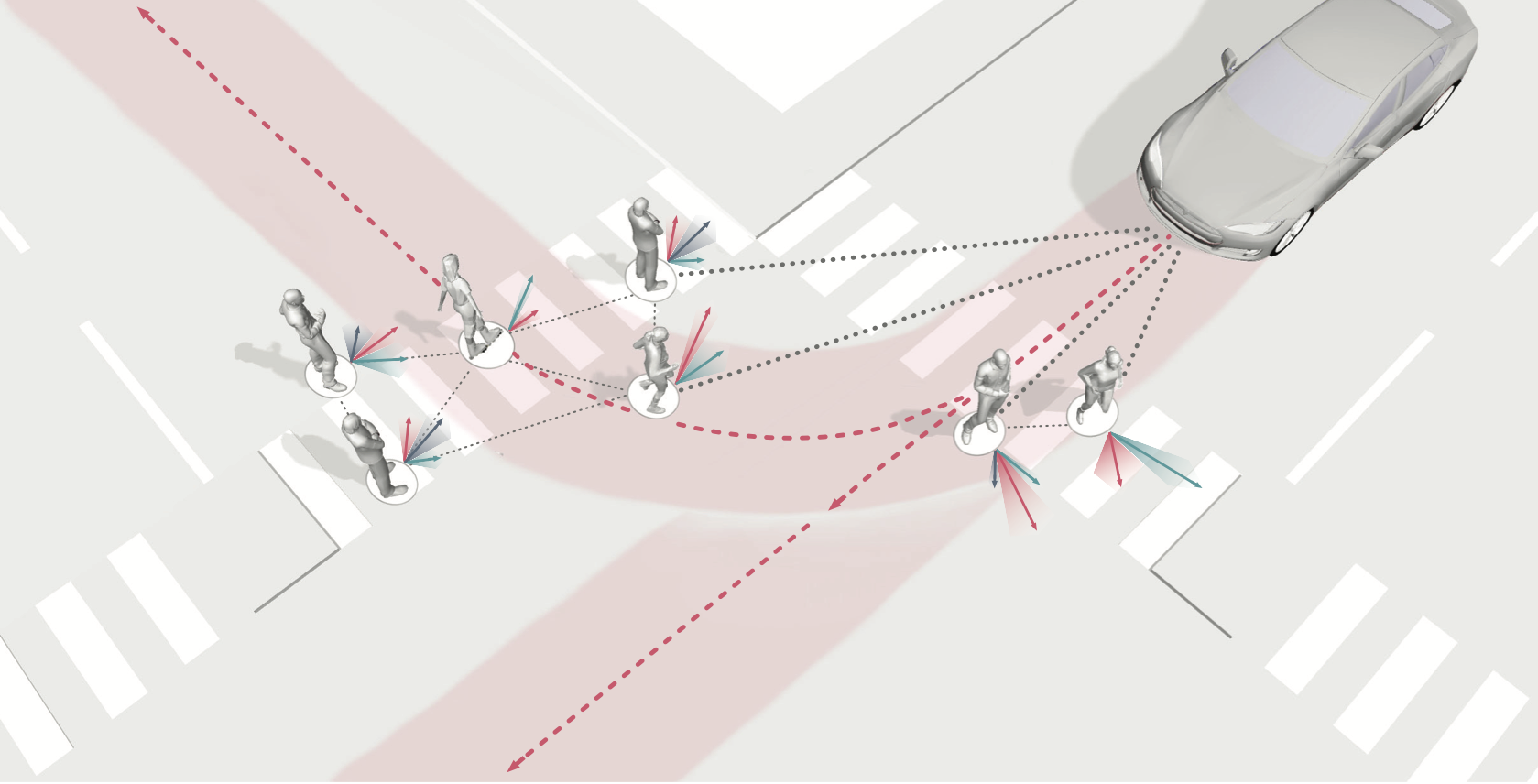
Merging into traffic is one of the most common day-to-day maneuvers we perform as drivers, yet still poses a major problem for self-driving vehicles. The reason that humans can naturally navigate through many social interaction scenarios, such as merging in traffic, is that they have an intrinsic capacity to reason about other people’s intents, beliefs, and desires, using such reasoning to predict what might happen in the future and make corresponding decisions¹. However, many current autonomous systems do not use such proactive reasoning, which leads to difficulties when deployed in the real world. For example, there have been numerous instances of self-driving vehicles failing to merge into traffic, getting stuck in intersections, and making unnatural decisions that confuse others. As a result, imbuing autonomous systems with the ability to reason about other agents’ actions could enable more informed decision making and proactive actions to be taken in the presence of other intelligent agents, e.g., in human-robot interaction scenarios. Indeed, the ability to predict other agents’ behaviors (also known as multi-agent behavior prediction) has already become a core component of modern robotic systems. This holds especially true in safety-critical applications such as autonomous vehicles, which are currently being tested in the real world and targeting widespread deployment in the near future². The diagram below illustrates a scenario where predicting the motion of other agents may help inform an autonomous vehicle’s path planning and decision making. Here, an autonomous vehicle is deciding whether to stay put or continue driving, depending on surrounding pedestrian movement. The red paths indicate future navigational plans for the vehicle, depending on its eventual destination.

At a high level, trajectory forecasting is the problem of predicting the path (trajectory) \(y\) that some sentient agent (e.g., a bicyclist, pedestrian, car driver, or bus driver) will move along in the future given the trajectory \(x\) that agent moved along in the past. In scenarios with multiple agents, we are also given their past trajectories, which can be used to infer how they interact with each other. Trajectories of length \(T\) are usually represented as a sequence of positional waypoints \(\{(p_1, p_2)_i\}_{i=1...T}\) (e.g., GPS coordinates). Since we aim to make good predictions, we evaluate methods by some metric that compares the predicted trajectory \(\widehat{y}\) against the actual trajectory the agent takes (denoted earlier as \(y\)).

In this post, we will dive into methods for trajectory forecasting, building a taxonomy along the way that organizes approaches by their methodological choices and output structures. We will discuss common evaluation schemes, present new ones, and suggest ways to compare otherwise disparate approaches. Finally, we will highlight shortcomings in existing methods that complicate their integration in downstream robotic use cases. Towards this end, we will present a new approach for trajectory forecasting that addresses these shortcomings, achieves state-of-the-art experimental performance, and enables new avenues of deployment on real-world autonomous systems.

1. Methods for Multi-Agent Trajectory Forecasting

There are many approaches for multi-agent trajectory forecasting, ranging from classical, physics-based models to deterministic regressors to generative probabilistic models³. To explore them in a structured manner, we will first group methods by the assumptions they make followed by the technical approaches they employ, building a taxonomy of trajectory forecasting methodologies along the way.

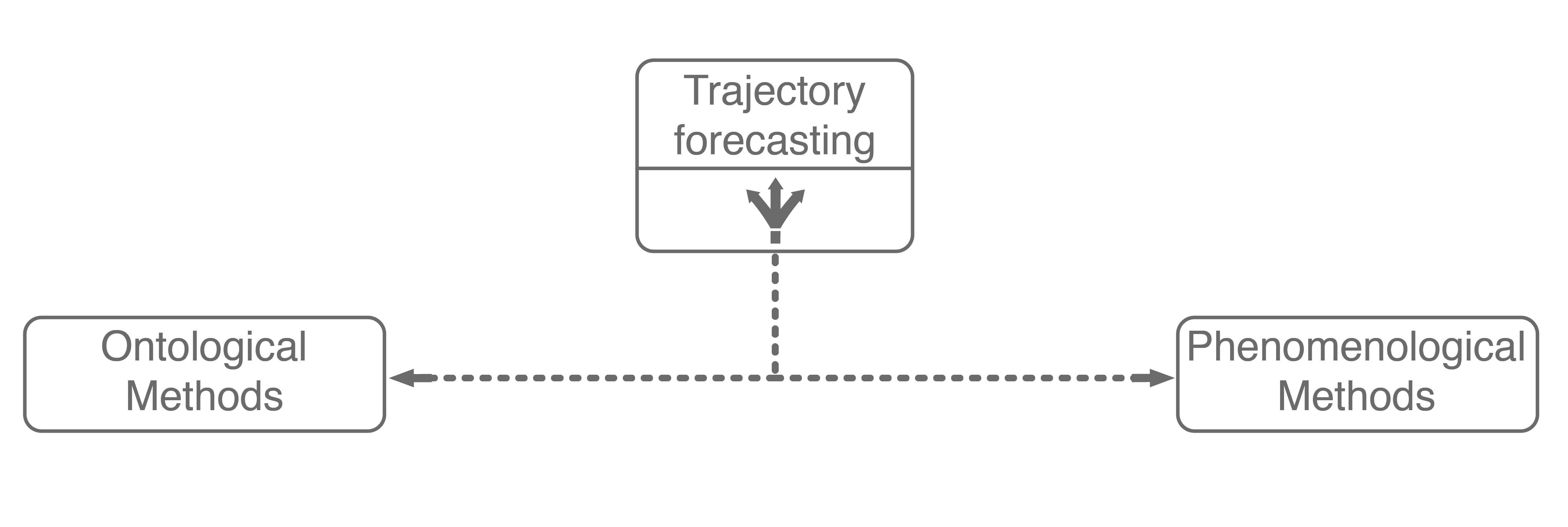
The first major assumption that approaches make is about the structure, if any, the problem possesses. In trajectory forecasting, this is manifested by approaches being either ontological or phenomenological. Ontological approaches (sometimes referred to as theory of mind) generally postulate (assume) some structure about the problem, whether that be a set of rules that agents follow or rough formulations of agents’ internal decision-making schemes. Phenomenological approaches do not make such assumptions, instead relying on a wealth of data to gleam agent behaviors without reasoning about underlying motivations.

1.1. Ontological Approaches

One of the simplest (and sometimes most effective) approaches for trajectory forecasting is classical mechanics. Usually, one assumes that they have a model that can predict the agent’s future state (also known as a dynamics model). With a dynamics model, one can predict the state (e.g., position, velocity, acceleration) of the agent several timesteps into the future. Such a simple approach is remarkably powerful, sometimes outperforming state-of-the-art approaches on real-world pedestrian modeling tasks⁴. However, pure dynamics integration alone does not account for the topology of the environment or interactions among agents, both of which are dominant effects. There have since been many approaches that mathematically formulate and model these interactions, exemplary methods include the intelligent driver model, MOBIL model, and Social Forces model.

More recently, inverse reinforcement learning (IRL) has emerged as a major ontological approach for trajectory forecasting. Given a set of agent trajectories in a scene \(\xi\), IRL attempts to learn the behavior and motivations of the agents. In particular, IRL formulates the motivation of an agent (e.g., crossing a sidewalk or turning right) with a mathematical formula, referred to as the reward function, shown below.

\[R(s) = w^T \phi(s),\]

where \(R(s)\) refers to the reward value at a specific state \(s\) (e.g., position, velocity, acceleration), \(w\) is a set of weights to be learned, and \(\phi(s)\) is a set of extracted features that characterize the state \(s\). Thus, the IRL problem is to find the best weights \(w\). The main idea here is that solving a reinforcement learning problem with a successfully-learned reward function would yield a policy that matches \(\xi\), the original agent trajectories.

Unfortunately, there can be many such reward functions under which the original demonstrations are recovered. Thus, we need a way to choose between possible reward functions. A very popular choice is to pick the reward function with maximum entropy. This follows the principle of maximum entropy, which states that the most appropriate distribution to model a given set of data is the one with highest entropy among all feasible possibilities⁵. A reason why one would want to do this is that maximizing entropy minimizes the amount of prior information built into the model; there is less risk of overfitting to a specific dataset. This is named Maximum Entropy (MaxEnt) IRL, and has seen widespread use in modeling real-world navigation and driving behaviors.

To encode this maximum entropy choice into the IRL formulation from above, trajectories with higher rewards are valued exponentially more. Formally,

\[p(\xi | w) \propto \exp \left(\sum_{s \in \xi} R(s)\right) = \sum_{s \in \xi} w^T \phi(s).\]

This distribution over paths also gives us a policy which can be sampled from. Specifically, the probability of an action is weighted by the expected exponentiated rewards of all trajectories that begin with that action.

Wrapping up, ontological approaches provide a structured method for learning how sentient agents make decisions. Due to their strong structural assumptions, they are both very sample-efficient (there are not many parameters to learn), computationally-efficient to optimize, and generally easier to pair with decision making systems (e.g., game theory). However, these strong structural assumptions also limit the maximum performance that an ontological approach may achieve. For example, what if the expert’s actual reward function was non-linear, had different terms than the assumed reward function, or was non-Markovian (i.e., had a history dependency)? In these cases, the assumed model would necessarily underfit the observed data. Further, data availability is growing at an exponential rate, with terabytes of autonomous driving data publicly being released every few months (companies have access to orders of magnitude more internally). With so much data, it becomes natural to consider phenomenological approaches⁶, which form the other main branch of our trajectory forecasting taxonomy.

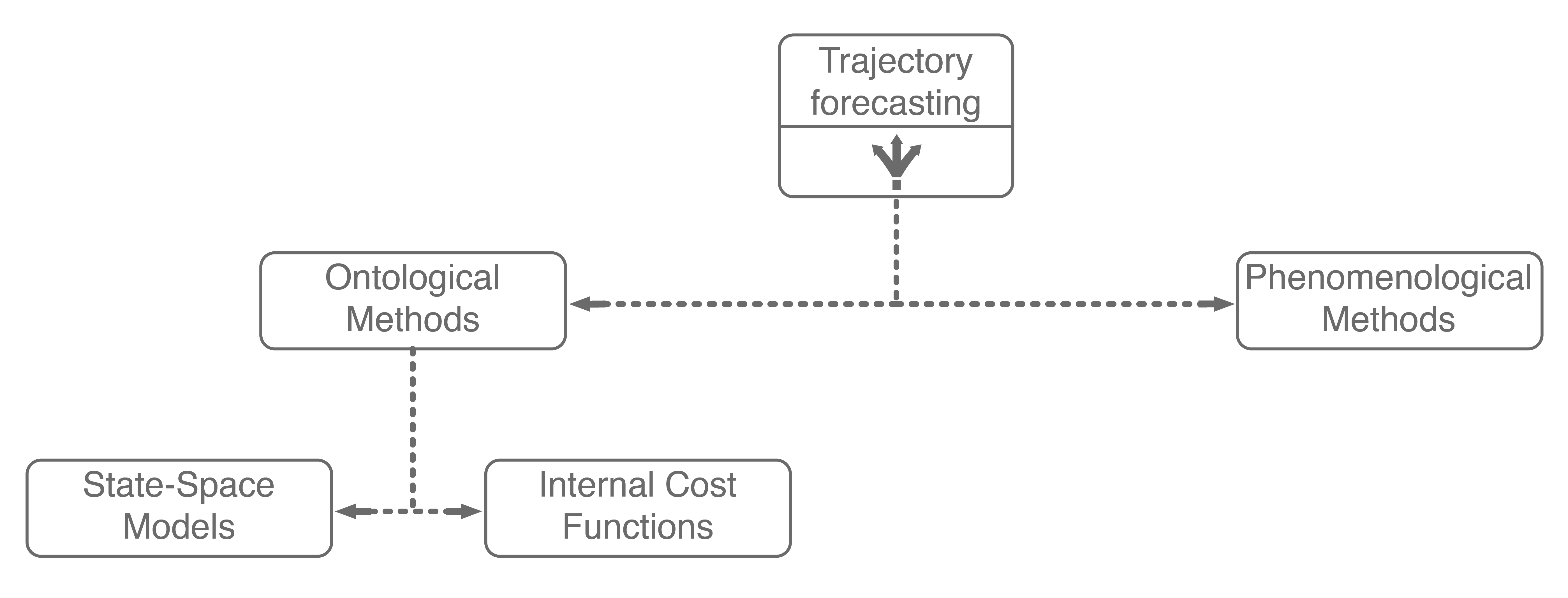
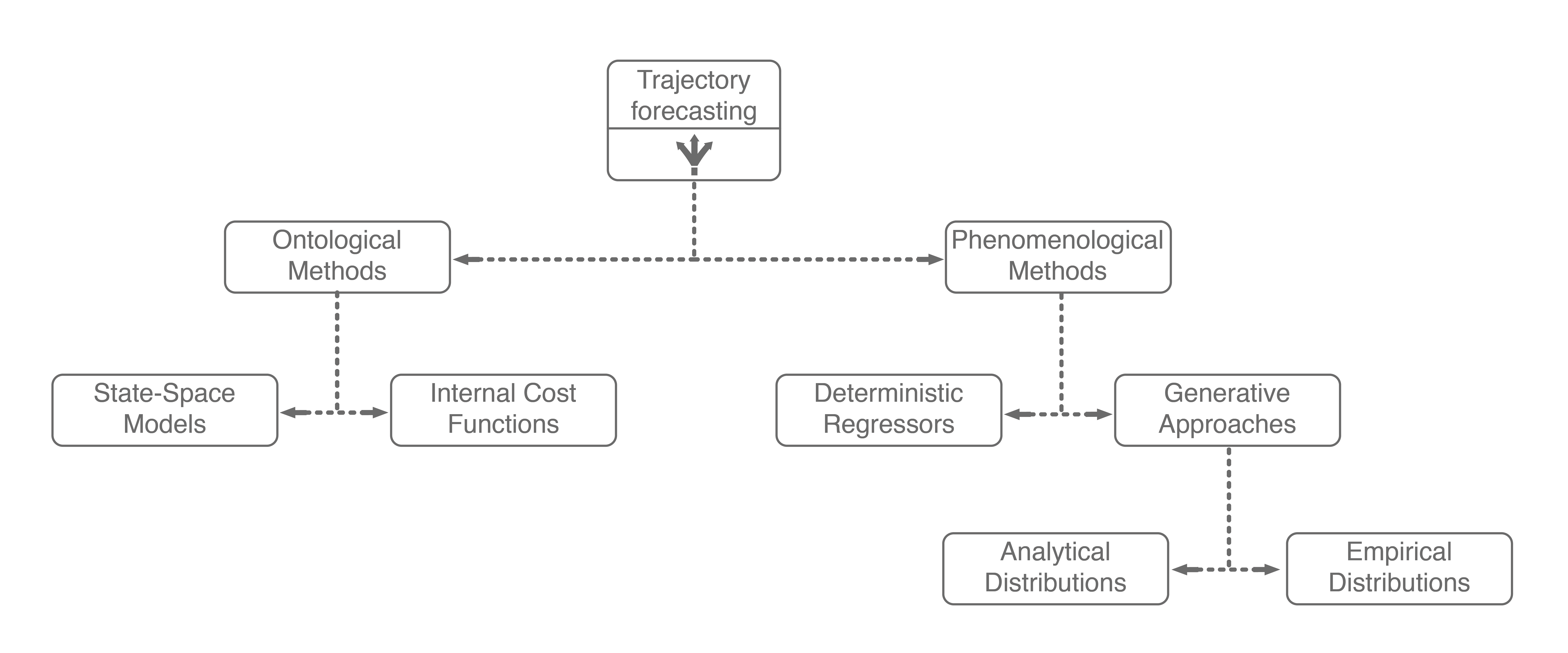
Including these two ontological approaches in our trajectory forecasting taxonomy yields the above tree. Next, we will dive into mainline phenomenological approaches.

1.2. Phenomenological Approaches

Phenomenological approaches are methods that make minimal assumptions about the structure of agents’ decision-making process. Instead, they rely on powerful general modeling techniques and a wealth of observation data to capture the kind of complexity encountered in environments with multiple interacting agents.

There have been a plethora of data-driven approaches for trajectory forecasting, mainly utilizing regressive methods such as Gaussian Process Regression (GPR)⁷ and deep learning, namely Long Short-Term Memory (LSTM) networks⁸ and Convolutional Neural Networks (CNNs)⁹, to good effect. Of these, LSTMs generally outperform GPR methods and are faster to evaluate online. As a result, they are commonly found as a core component of human trajectory models¹⁰. The reason why LSTMs perform well is that they are a purpose-built deep learning architecture for modeling temporal sequence data. Thus, practitioners usually model trajectory forecasting as a time series prediction problem and apply LSTM networks.

While these methods have enjoyed strong performance, there is a subtle point that limits their application to safety-critical problems such as autonomous driving: they only produce a single deterministic trajectory forecast. Safety-critical systems need to reason about many possible future outcomes, ideally with the likelihoods of each occurring, to make safe decisions online. As a result, methods that simultaneously forecast multiple possible future trajectories have been sought after recently.

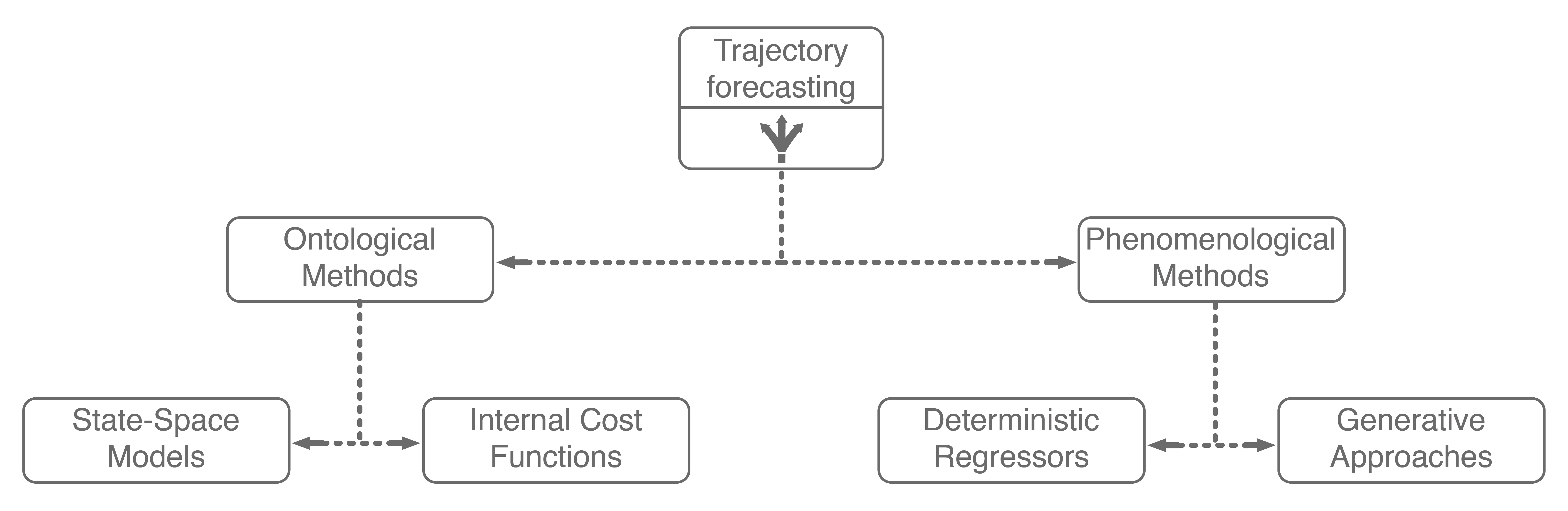
Generative approaches in particular have emerged as state-of-the-art trajectory forecasting methods due to recent advancements in deep generative models¹¹. Notably, they have caused a paradigm shift from focusing on predicting the single best trajectory to producing a distribution of potential future trajectories. This is advantageous in autonomous systems as full distribution information is more useful for downstream tasks, e.g., motion planning and decision making, where information such as variance can be used to make safer decisions. Most works in this category use a deep recurrent backbone architecture (like an LSTM) with a latent variable model, such as a Conditional Variational Autoencoder (CVAE), to explicitly encode multimodality¹², or a Generative Adversarial Network (GAN) to implicitly do so¹³. Common to both approach styles is the need to produce position distributions. GAN-based models can directly produce these and CVAE-based recurrent models usually rely on a bivariate Gaussian or bivariate Gaussian Mixture Model (GMM) to output position distributions. Including the two in our taxonomy balances out the right branch.

The main difference between GAN-based and CVAE-based approaches is in the form of their resulting output distribution. At a high level, GANs are generative models that generate data which, in aggregate, match the distribution \(p(y)\) of its training dataset \(\mathcal{D}\). They achieve this by learning to map samples \(x\) from a known distribution \(K\) to samples \(y\) of an unknown distribution \(\mathcal{D}\) for which we have samples, i.e., the training dataset. Intuitively, this is very similar to inverse transform sampling, which is a method for generating samples from any probability distribution given its cumulative distribution function. This is roughly illustrated below, where samples from a simple uniform distribution are mapped to a standard Gaussian distribution.

Sourced from this excellent article on understanding GANs.

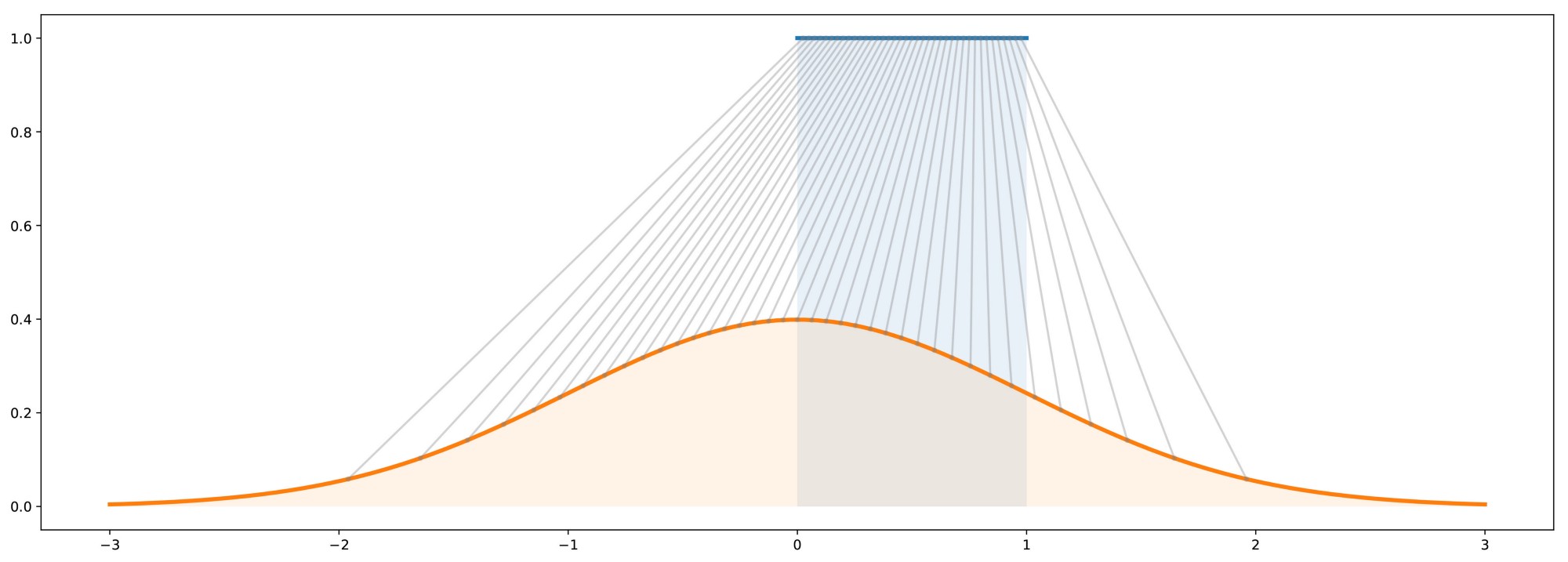
Thus, GANs can be viewed as learning an inverse transformation which maps a sample of a “simple” random variable \(x \sim p(x)\) to a sample of a “complex” random variable \(y \sim p(y \mid x)\) (conditioned on \(x\) because that is the value being mapped to \(y\)). Thinking about this from the perspective of trajectory forecasting, \(x\) is usually the trajectory history of the agent, information about neighboring agents, environmental information, etc. and \(y\) is the trajectory forecast we are looking to output. Thus, it makes sense that one would want to produce predictions \(y \sim p(y \mid x)\) conditioned on past observations \(x\). However, this sampling-based structure also means that GANs can only produce empirical, and not analytical, distributions. Specifically, obtaining statistical properties like the mean and variance from a GAN can only be done approximately, through repeated sampling.

On the other hand, CVAEs tackle the problem of representing \(p(y \mid x)\) by decomposing it into subcomponents specified by the value of a latent variable \(z\). Formally,

\[p(y \mid x) = \sum_z p(y \mid x, z) p(z \mid x).\]

Note that the sum in the above equation implies that \(z\) is discrete (has finitely-many values). The latent variable \(z\) can also be continuous, but there is work showing that discrete latent spaces lead to better performance (this also holds true for trajectory forecasting)¹⁴, so for this post we will only concern ourselves with a discrete \(z\). By decomposing \(p(y \mid x)\) in this way, one can produce an analytic output distribution. This is very similar to GMMs, which also decompose their desired \(p(\text{data})\) distribution in this manner to produce an analytic distribution. This completes our taxonomy, and broadly summarizes current approaches for multi-agent trajectory forecasting.

With such a variety of approach styles, how do we know which is best? How can we determine if, for example, an approach that produces an analytic distribution outperforms a deterministic regressor?

2. Benchmarking Performance in Trajectory Forecasting

With such a broad range of approaches and output structures, it can be difficult to evaluate progress in the field. Even phrasing the question introduces biases towards methods. For example, asking the following excludes generative or probabilistic approaches: Given a trajectory forecast \(\{\widehat{y}_1, ..., \widehat{y}_T\}\) and the ground truth future trajectory \(\{y_1, ..., y_T\}\), how does one evaluate how “close” the forecast is to the ground truth? We will start with this question, even if it is exclusionary for certain classes of methods.

Illustrated above, one of the most common ways is to directly compare them side-by-side, i.e., measure how far \(\widehat{y}_i\) is from \(y_i\) for each \(i\) and then average these distances to obtain the average error over the prediction horizon. This is commonly known as Average Displacement Error (ADE) and is usually reported in units of length, e.g., meters:

\[ADE(\widehat{y}, y) = \frac{1}{T} \sum_{i=1}^T ||\widehat{y}_i - y_i||_2^2.\]

Often, we are also interested in the displacement error of only the final predicted point, illustrated below (in particular, only \(\widehat{y}_3\) and \(y_3\) are compared).

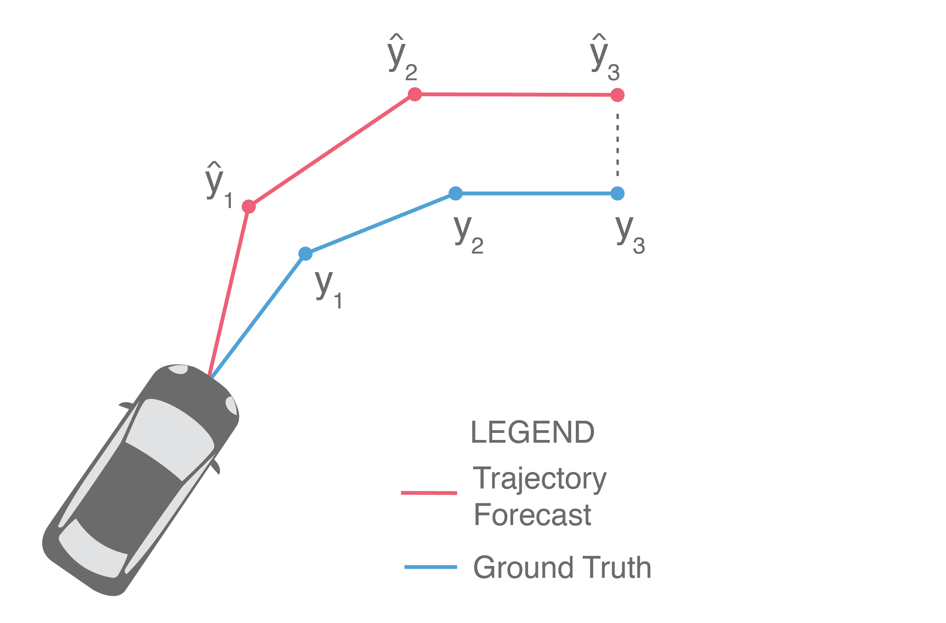
This provides a measure of a method’s error at the end of the prediction horizon, and is frequently referred to as Final Displacement Error (FDE). It is also usually reported in units of length.

\[FDE(\widehat{y}, y) = || \widehat{y}_T - y_T ||_2^2.\]

ADE and FDE are the two main metrics used to evaluate deterministic regressors. While these metrics are natural for the task, easy to implement, and interpretable, they generally fall short in capturing the nuances of more sophisticated methods (see more on this below). It is for this reason, perhaps, that they have historically led to somewhat inconsistent reported results. For instance, there are contradictions between the results reported by the same authors in Gupta et al. (2018) and Alahi et al. (2016). Specifically, in Table 1 of Alahi et al. (2016), Social LSTM convincingly outperforms a baseline LSTM without pooling. However, in Table 1 of Gupta et al. (2018), Social LSTM is actually worse than the same baseline on average. Further, the values reported by Social Attention in Vemula et al. (2018) seem to have unusually high ratios of FDE to ADE. Nearly every other published method has FDE/ADE ratios around \(2-3\times\) whereas Social Attention’s are around \(3-12\times\). Social Attention’s reported errors on the UCY - University dataset are especially striking, as its FDE after 12 timesteps is \(3.92\), which is \(12\times\) its ADE of \(0.33\). This would make its prediction error on the other 11 timesteps essentially zero.

As mentioned earlier, safety-critical systems need to reason about many possible future outcomes, ideally with the likelihoods of each occurring, so that safe decision-making can take place which considers a whole range of possible futures. In this context, ADE and FDE are unsatisfactory because they focus on evaluating a single trajectory forecast. This leaves the following question: How do we evaluate generative approaches which produce many forecasts simultaneously, or even full distributions over forecasts?

Given the ground truth future trajectory \(\{y_1, ..., y_T\}\) and the ability to sample trajectory forecasts \(\{\widehat{y}_1, ..., \widehat{y}_T\}\), how does one evaluate how “good” the samples are with respect to the ground truth? One initial idea, illustrated below, is to sample \(N\) forecasts from the model and then return the performance of the best forecast. This is usually referred to as Best-of-N (BoN), along with the underlying performance metric used. For example, a Best-of-N ADE metric is illustrated below, since \(N = 3\) and we measure the ADE of the best forecast, i.e., the forecast with minimum ADE.

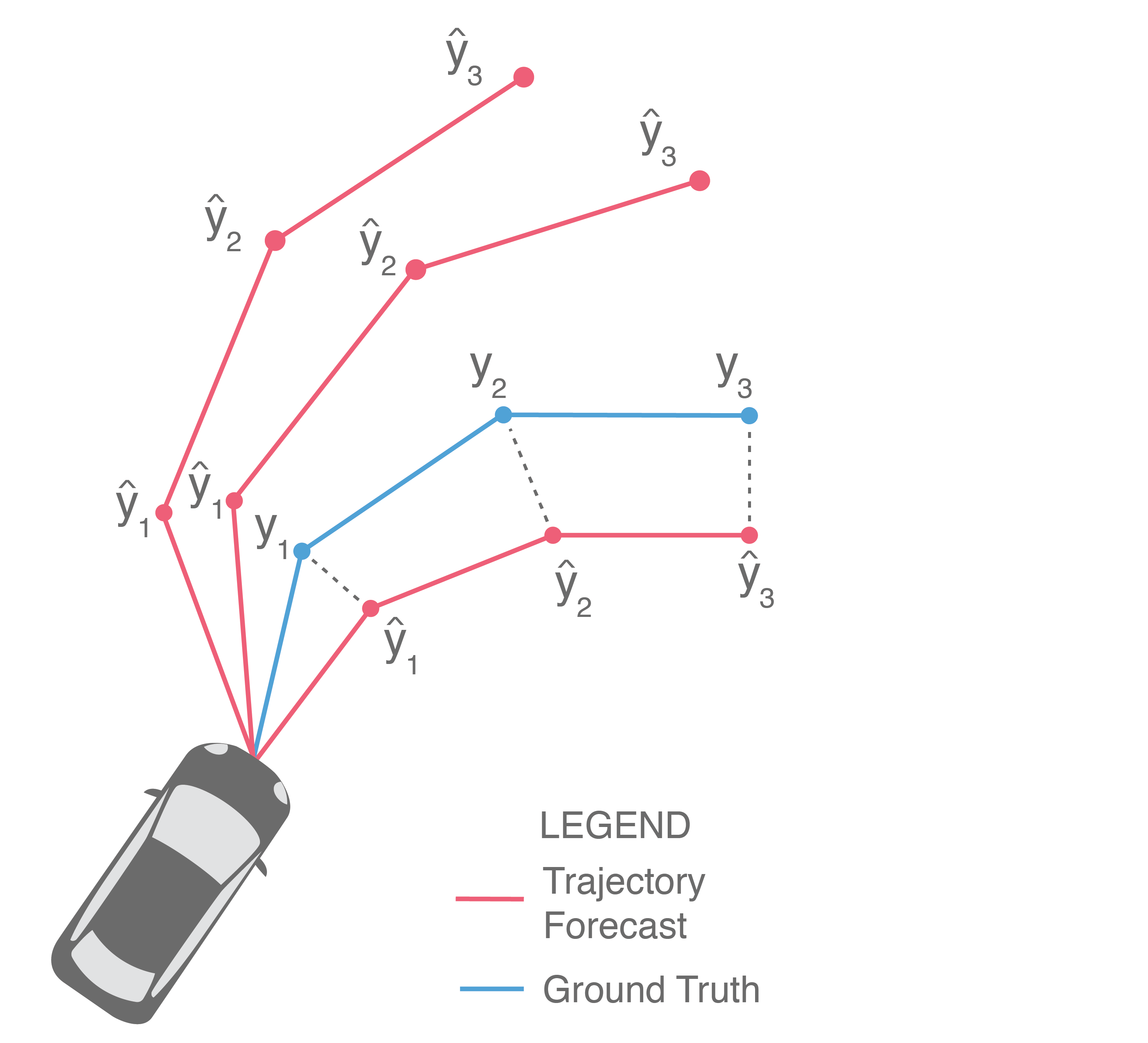
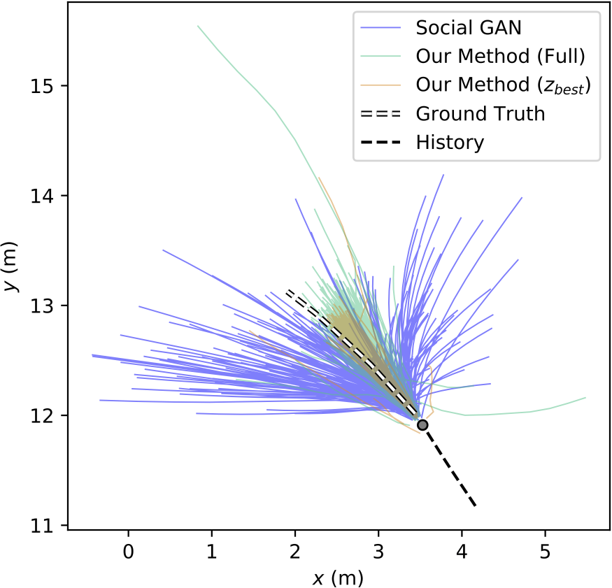
This is the main metric used by generative methods that produce empirical distributions, such as GAN-based approaches. The idea behind this evaluation scheme is to identify if the ground truth is near the forecasts produced by a few samples from the model (\(N\) is usually chosen to be small, e.g., \(20\)). Implicitly, this evaluation metric selects one sample as the best prediction and then evaluates it with the ADE/FDE metrics from before. However, this is inappropriate for autonomous driving because it requires knowledge of the future (in order to select the best prediction) and it is unclear how to relate BoN performance to the real world. It is also difficult to objectively compare methods using BoN because approaches that produce wildly different output samples may yield similar BoN metric values, as illustrated below.

This is a figure from our recent trajectory forecasting work at ICCV 2019 which compares versions of our method, the Trajectron, with that of the (generative, empirical) Social GAN. If one were to use a Best-of-N ADE or FDE metric on these outputs, both methods might perform similarly even though Social GAN produces outputs with significantly higher variance.

To address these shortcomings in the Best-of-N metric, we proposed a new evaluation scheme for generative, empirical methods in our recent ICCV 2019 paper¹⁵. Illustrated below, one starts by sampling many trajectories (\(\sim 10^3\), to obtain a representative set of outputs) from the methods being compared. A Kernel Density Estimate (KDE; a statistical tool that fits a probability density function to a set of samples) is then fit at each prediction timestep to obtain a probability density function (pdf) of the sampled positions at each timestep. From these pdfs, we compute the mean log-likelihood of the ground truth trajectory. This metric is called the KDE-based Negative Log-Likelihood (KDE NLL) and is reported in logarithmic units, i.e., nats.

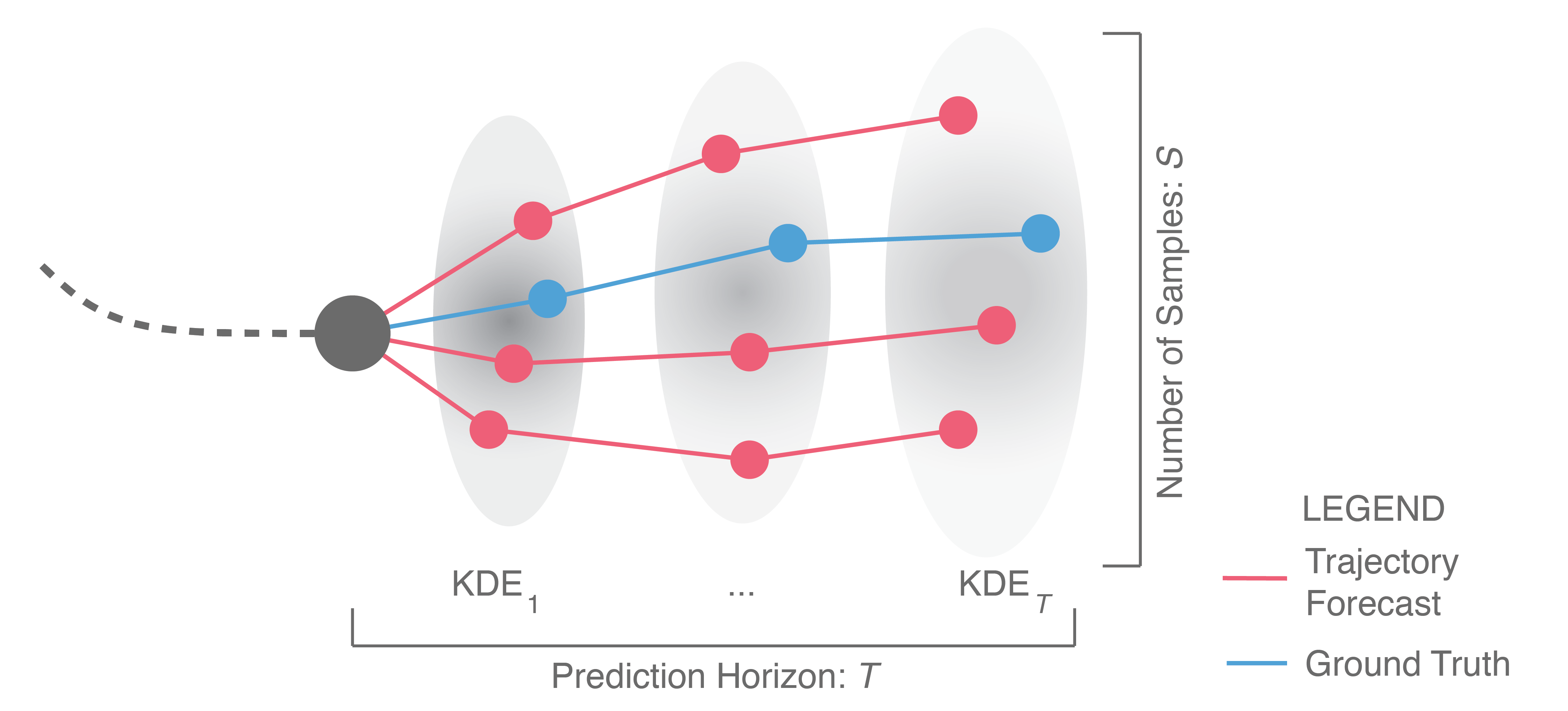
KDE NLL does not suffer from the same downsides that BoN does, as (1) methods with wildly different outputs will yield wildly different KDEs, and (2) it does not require looking into the future during evaluation. Additionally, it fairly estimates a method’s NLL without any assumptions on the method’s output distribution structure; both empirical and analytical distributions can be sampled from. Thus, KDE NLL can be used to compare methods across taxonomy groups.

While KDE NLL can compare generative methods, deterministic lines of work are still disparate in their metrics and evaluating across the generative/deterministic boundary remains difficult. We also tried to tackle this in our 2019 ICCV paper, settling on the following comparison where we compared boxplots of generative methods alongside ADE and FDE (shown below) values from deterministic methods. The methods were trained and evaluated on the ETH and UCY pedestrian datasets, containing thousands of rich multi-human interaction scenarios.

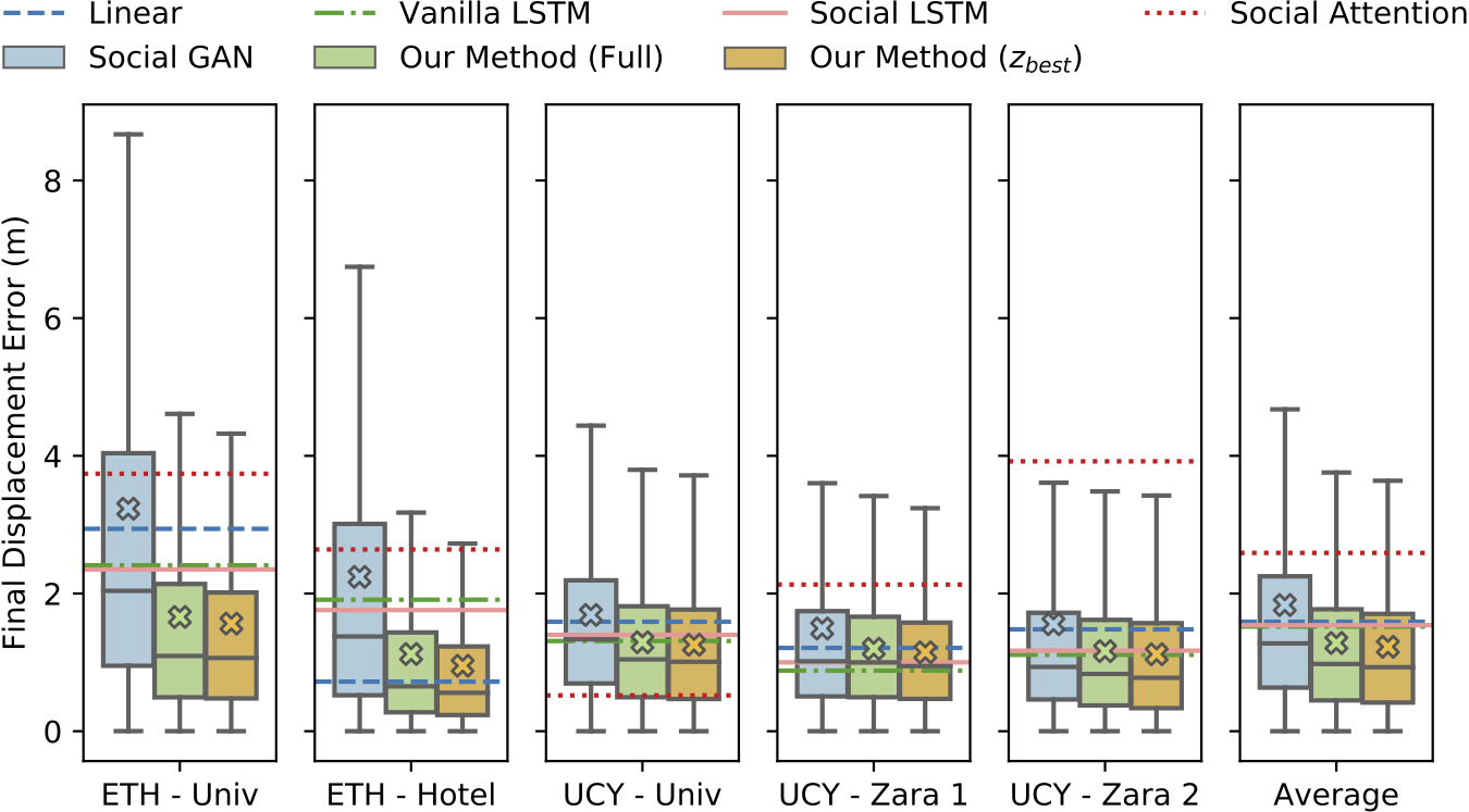
Even though we created the above figure, it is not immediately obvious how to interpret it. Should one compare means and medians? Should one try statistical hypothesis tests between error distributions and mean error values from deterministic values? Unfortunately, using boxplots (as we did in our ICCV work) disregards the possibility for multimodal error distributions (i.e., a distribution with many peaks). Another possibility may be to let dataset curators decide the most relevant metrics for their dataset, e.g., the nuScenes dataset (a large-scale autonomous driving dataset from nuTonomy) has a prediction challenge with specific evaluation metrics. This may yield proper comparisons for a specific dataset, but it still allows for biases towards certain kinds of approaches and makes it difficult to compare approaches across datasets. For example, evaluating generative approaches with ADE and FDE ignores variance, which may make two different methods appear to perform the same (see trajectory samples from Trajectron vs. Social GAN in the earlier qualitative plot).

Overall, there is still much work to be done in standardizing metrics across approach styles and datasets. Some open questions in this direction are:

• Do we really care equally about each waypoint in ADE? We know that forecasts degrade with prediction horizon, so why not focus on earlier or later prediction points more?
• Why even aggregate displacement errors? We could compare the distribution of displacement errors per timestep, e.g., using a statistical hypothesis test like the t-test.
• For methods that also produce variance information, why not weigh their predictions by \(1/\text{Var}(\widehat{y}_i)\)? This would enable methods to specify their own uncertainties and be rewarded, e.g., if they are making bad predictions in weird scenarios, but alerting that they are uncertain.
• Since these forecasts are ultimately being used for decision making and control, a control-aware metric would be useful. For instance, we may want to evaluate an output’s control feasibility by how many control constraint violations there are on average over the course of a forecast.

We will now discuss our newly-released method for trajectory forecasting that addresses these cross-taxonomy evaluation quandaries by being explicitly designed to be simultaneously comparable with both generative and deterministic approaches. Further, this approach also addresses how to include system dynamics and additional data sources (e.g., maps, camera images, LiDAR point clouds) such that its forecasts are all physically-realizable by the modeled agent and consider the topology of the surrounding environment.

3. Trajectron++: Dynamically-Feasible Trajectory Forecasting With Heterogeneous Data

As mentioned earlier, nearly every trajectory forecasting method directly produces positions as their output. Unfortunately, this output structure makes it difficult to integrate with downstream planning and control modules, especially since purely-positional trajectory predictions do not respect dynamics constraints, e.g., the fact that a car cannot move sideways, which could lead to models producing trajectory forecasts that are unrealizable by the underlying control variables, e.g., predicting that a car will move sideways.

Towards this end, we have developed Trajectron++, a significant addition to the Trajectron framework, that addresses this shortcoming. In contrast to existing approaches, Trajectron++ explicitly accounts for system dynamics, and leverages heterogeneous input data (e.g., maps, camera images, LIDAR point clouds) to produce state-of-the-art trajectory forecasting results on a variety of large-scale real-world datasets and agent types.

Trajectron++ is a graph-structured generative (CVAE-based) neural architecture that forecasts the trajectories of a general number of diverse agents while incorporating agent dynamics and heterogeneous data (e.g., semantic maps). It is designed to be tightly integrated with robotic planning and control frameworks; for example, it can produce predictions that are optionally conditioned on ego-agent motion plans. At a high level, it operates by first creating a spatiotemporal graph representation of a scene from its topology. Then, a similarly-structured deep learning architecture is generated that forecasts the evolution of node attributes, producing agent trajectories. An example of this is shown below.

A scene around the ego-vehicle in the nuScenes dataset is shown. From the distances between different agents (e.g., pedestrians, cars), a spatiotemporal graph is built (left) which then dictates how the corresponding neural network architecture (right) is constructed. The architecture models agents by encoding the agent’s history and local interactions (edges).

We will focus on two aspects of our model, each of which address one of the problems we previously highlighted (considering dynamics and comparing across the trajectory forecasting taxonomy).

3.1. Incorporating System Dynamics into Generative Trajectory Forecasting

One of the main contributions of Trajectron++ is presenting a method for producing dynamically-feasible output trajectories. Most CVAE-based generative methods capture fine-grained uncertainty in their outputs by producing the parameters of a bivariate Gaussian distribution (i.e., its mean and covariance) and then sampling position waypoints from it. However, this direct modeling of position is ignorant of an agent’ governing dynamics and relies on the neural network architecture to learn dynamics.

While neural networks can do this, we are already good at modeling the dynamics of many systems, including pedestrians (as single integrators) and vehicles (e.g., as dynamically-extended unicycles)¹⁶. Thus, Trajectron++ instead focuses on forecasting distributions of control sequences which are then integrated through the agent’s dynamics to produce positions. This ensures that the output trajectories are physically realizable as they have associated control strategies. Note that the full distribution itself is integrated through the dynamics. This can be done for each latent behavior mode via the Kalman Filter prediction equations (for linear dynamics models) or the Extended Kalman Filter prediction equations (for nonlinear dynamics models).

As a bonus, adding agent dynamics to the model yields noticeable performance improvements across all evaluation metrics. Broadly, this makes sense as the model’s loss function (the standard Evidence Lower Bound CVAE loss) can now be directly specified over the desired quantity (position) while still respecting dynamic constraints.

3.2. Leveraging Heterogeneous Data Sources

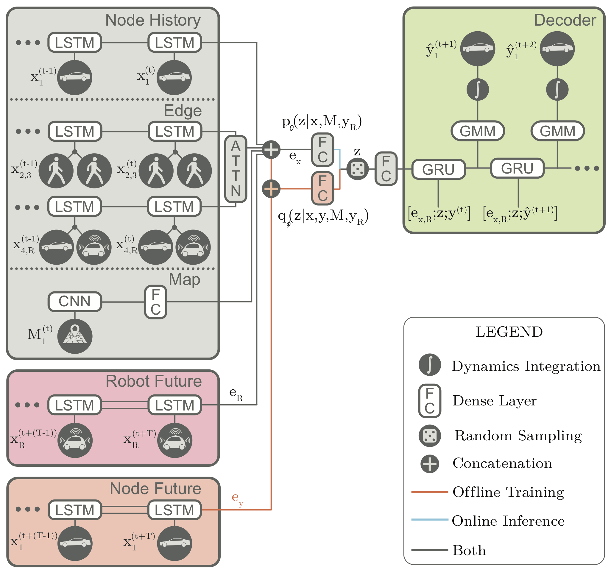
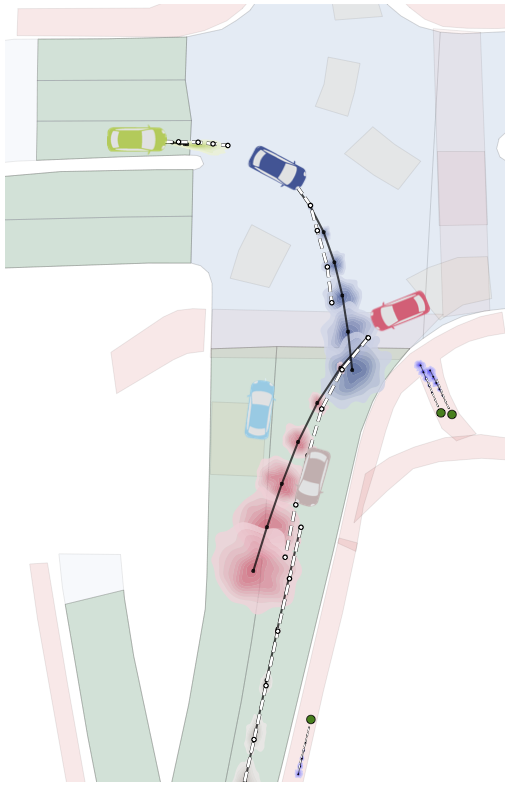
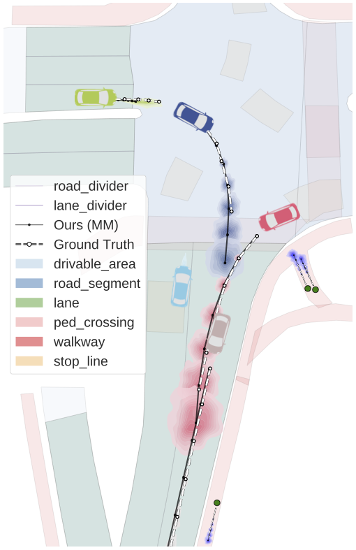
An additional feature of Trajectron++ is its ability to combine data from a variety of sources to produce forecasts. In particular, the presence of a single backbone representation vector, denoted \(e_x\) in the above architecture diagram, enables for the seamless addition of new data via concatenation. To illustrate this, we show the benefits of including high-definition maps in the figure below. In it, we can see that the model is able to improve its predictions in turns, better reflecting the local lane geometry.

Left: Without map information, the model tends to undershoot turns. Right: Encoding a local map of the agent's surroundings notably increases Trajectron++'s accuracy and confidence in turns. It is able to use semantic labels (shown in color) to reason about where agents can go.

3.3. Simultaneously Producing Both Generative and Deterministic Outputs

A key feature of the Trajectron and Trajectron++ models is their combination of a CVAE with a Gaussian output. Specifically, the “GMM” in the above architecture diagram only has one component, i.e., it is just a multivariate Gaussian. Thus, the model’s overall output is

\[p(y \mid x) = \sum_z p(y \mid x, z) p(z \mid x) = \sum_z p(z \mid x) p(y \mid x, z) = \sum_z \pi_z(x) \mathcal{N}(y; \mu(x, z), \Sigma(x, z)),\]

which is the definition of a GMM! Thus, each component \(z\), which is meant to model high-level latent behaviors, ends up specifying a set of parameters for a Gaussian output distribution over control variables. With such a form, we can easily produce both generative and deterministic outputs. The following are the main four outputs that Trajectron++ can produce.

• Most Likely (ML): This is the model’s deterministic and most-likely single output. The high-level latent behavior mode and output trajectory are the modes of their respective distributions, where

\[z_\text{mode} = \arg \max_z p(z \mid x), \ \ \ \ \ \ \ \ y = \arg \max_{y} p(y \mid x, z_\text{mode}).\]

• \(z_{\text{mode}}\): Predictions from the model’s most-likely high-level latent behavior mode, where

\[z_\text{mode} = \arg \max_z p(z \mid x), \ \ \ \ \ \ \ \ y \sim p(y \mid x, z_\text{mode}).\]

• Full: The model’s full sampled output, where \(z\) and \(y\) are sampled sequentially according to

\[z \sim p(z \mid x), \ \ \ \ \ \ \ \ y \sim p(y \mid x, z).\]

• Distribution: Due to the use of a discrete Categorical latent variable and Gaussian output structure, the model can provide an analytic output distribution by directly computing

\[p(y \mid x) = \sum_z p(y \mid x, z) p(z \mid x).\]

Thus, to compare against deterministic methods we use Trajectron++’s most-likely prediction with ADE and FDE. To compare against generative empirical or analytical methods, we use any of \(z_{\text{mode}}\), Full, or Distribution with KDE NLL. In summary, Trajectron++ can be directly compared to any method that produces either a single trajectory or a distribution thereof.

Trajectron++ serves as a first step along a broader research thrust to better integrate modern trajectory forecasting approaches with robotic planning, decision making, and control. In particular, we are broadening our focus from purely minimizing benchmark error to also considering the advancements needed to successfully deploy modern trajectory forecasting methods to the real world, where properties like runtime, scalability, and data dependence play increasingly important roles. This in turn raises further research questions, for example:

• What output representation best suits downstream planners? Predicting positional information alone makes it difficult to use some planning, decision making, and control algorithms.
• What is required of perception? How difficult is it to obtain the desired input information?

Some research groups are already tackling these types of questions¹⁷, viewing trajectory forecasting as a modular component that is integrated with perception, planning, and control modules.

4. Conclusion

Now that there is a large amount of publicly-available trajectory forecasting data, we have crossed the threshold where data-driven, phenomenological approaches generally surpass the performance of ontological methods. In particular, recent advances in deep generative modeling have brought forth a probabilistic paradigm shift in multi-agent trajectory forecasting, leading to new considerations about evaluation metrics and downstream use cases.

In this post, we constructed a taxonomy of existing mainline approaches (e.g., Social Forces and IRL) and newer research (e.g., GAN-based and CVAE-based approaches), discussed their evaluation schemes and suggested ways to compare approaches across taxonomy groups, and highlighted shortcomings that complicate their integration in downstream robotic use cases. Towards this end, we present Trajectron++, a novel phenomenological trajectory forecasting approach that incorporates dynamics knowledge and the capacity for heterogeneous data inclusion. As a step towards the broader research thrust of integrating trajectory forecasting with autonomous systems, Trajectron++ produces dynamically-feasible trajectories in a wide variety of output formats depending on the specific downstream use case. It achieves state-of-the-art performance on both generative and deterministic benchmarks, and enables new avenues of deployment on real-world autonomous systems.

There are still many open questions, especially in terms of standard evaluation metrics, model interpretability, and broader architectural considerations stemming from future integration with downstream planning and control algorithms. This especially rings true now that deep learning approaches have outweighed others in popularity and performance, and are targeting deployment on real-world safety-critical robotic systems.

---

This blog post is based on the following paper:

• Trajectron++: Dynamically-Feasible Trajectory Forecasting With Heterogeneous Data by Tim Salzmann*, Boris Ivanovic*, Punarjay Chakravarty, and Marco Pavone.¹⁸

All of our code, models, and data are available here. If you have any questions, please contact Boris Ivanovic.

Acknowledgements

Many thanks to Karen Leung and Marco Pavone for comments and edits on this blog post, Matteo Zallio for visually communicating our ideas, and Andrei Ivanovic for proofreading.

1. Gweon and Saxe provide a good overview of this concept, commonly known as “theory of mind”, in this book chapter. ↩

2. For example, both Uber and Waymo provide safety reports discussing what they have learned from real-world testing as well as their strategies for developing safe self-driving vehicles that can soon operate among humans. ↩

3. An excellent recent review can be found in Rudenko et al. (2019). ↩

4. Examples include Schneider and Gavrila (2013) and Schöller et al. (2020). ↩

5. See Jaynes (1957a) and Jaynes (1957b) for more details. ↩

6. See Swamy et al. (2020) for a deeper dive into comparisons between ontological and phenomenological methods. ↩

7. E.g., Rasmussen and Williams (2006), Wang et al. (2008). ↩

8. E.g., Alahi et al. (2016), Morton et al. (2017), Vemula et al. (2018). ↩

9. E.g., Zeng et al. (2019), Casas et al. (2018), Jain et al. (2019), Casas et al. (2019) ↩

10. E.g., Alahi et al. (2016), Jain et al. (2016), Vemula et al. (2018). ↩

11. Especially Sohn et al. (2015) and Goodfellow et al. (2014). ↩

12. Here is a partial list of primarily CVAE-based methods: Lee et al. (2017), Schmerling et al. (2018), Ivanovic et al. (2018), Deo and Trivedi (2018), Sadeghian et al. (2018), Ivanovic and Pavone (2019), Rhinehart et al. (2019). ↩

13. Here is a partial list of primarily GAN-based methods: Gupta et al. (2018), Sadeghian et al. (2019), Kosaraju et al. (2019). ↩

14. E.g., Jang et al. (2017), Maddison et al. (2017), Moerland et al. (2017). ↩

15. Ivanovic and Pavone, The Trajectron: Probabilistic Multi-Agent Trajectory Modeling with Dynamic Spatiotemporal Graphs, IEEE/CVF International Conference on Computer Vision (ICCV) 2019. ↩

16. For more information, see Kong et al. (2015) and Paden et al. (2016). ↩

17. E.g., Weng et al. (2020), Zeng et al. (2019). ↩

18. * denotes equal contribution ↩